You run a small web service with a single worker. Each request needs about one millisecond of real work, and requests arrive at random from many users. You watch the dashboard while traffic grows: the worker is busy half the time, then eighty percent of the time, then ninety. It's natural to expect each request to get a little slower as the load goes up, in step with the load.
It doesn't work that way. At ninety percent busy a request still needs exactly one millisecond of work, but it now takes about ten milliseconds from the moment it arrives to the moment its answer goes out, a time that engineers call its latency. The extra nine milliseconds are spent waiting for a worker that's busy with someone else's request. Close to full, the waiting grows far faster than the load, and it lands hardest on the unluckiest requests, so the slowest one in a hundred can take several times as long as the average one. Adding more workers helps only until they start getting in each other's way. And when one page needs answers from a hundred other services, an answer that's slow one time in a hundred turns into the normal case.
All of this comes from one ingredient, a line of requests waiting for something shared, and it looks the same whether the shared thing is a worker, a lock, a database connection or a disk. The question for this chapter is: why does a service that isn't full already feel slow, and why do its slowest requests pay the most? We'll start by simulating that one worker so you can see the numbers for yourself, and then work out, step by step, where the waiting comes from and how to measure it honestly.
01One worker and a line of requests
1.1The server we'll simulate
Let's pin the server down so a script can play it. It has one worker, and each request needs one millisecond of work on average. That's its service time: how long the worker needs once it starts on a request. Requests arrive at random moments, so sometimes two show up almost together. A request that arrives while the worker is busy goes to the back of a line and waits there. That line is the queue, and a request's latency is the time it spends in the queue plus its service time.
The fraction of time the worker spends busy is its utilisation, written ρ (the Greek letter rho). If a request arrives every two milliseconds on average, that's half a request per millisecond, each one takes a millisecond, and the worker is busy half the time: ρ = 0.5. At nine requests per ten milliseconds, ρ = 0.9.
An average hides the unlucky requests, so the script reports two numbers for each run. The mean is the ordinary average latency. The p99 is found by sorting every request's latency from fastest to slowest and picking the one 99% of the way along, so 99 of every 100 requests finished faster than it and one in a hundred took longer. (Statisticians call it the 99th percentile.)
The script needs random numbers for the gaps between arrivals and for the service times. random.expovariate(rate) returns a random gap that averages 1/rate, mostly short and now and then long, which is the standard model for things that happen at random.
1.2Trying it: five load levels
Each pass through the loop in the script is one request. t_arrive += … moves the clock on to the next arrival. start = max(t_arrive, server_free) says the request starts when it has arrived and the worker is free, whichever comes later, and that one line is the whole queue. The request then takes a random service time, and its latency is its finish time minus its arrival time. The fixed seed makes every run print the same numbers, and 400,000 requests per row is enough to smooth out most of the luck.
import random

def simulate(utilisation, jobs=400_000, service_ms=1.0, seed=1):
    rng = random.Random(seed)
    arrive_rate = utilisation / service_ms           # jobs per ms
    t_arrive = 0.0; server_free = 0.0; lat = []
    for _ in range(jobs):
        t_arrive += rng.expovariate(arrive_rate)     # random arrivals
        start = max(t_arrive, server_free)           # wait if the server is busy
        service = rng.expovariate(1 / service_ms)    # random service, mean 1 ms
        server_free = start + service
        lat.append(server_free - t_arrive)
    lat.sort()
    return sum(lat) / len(lat), lat[int(0.99 * len(lat))]

print(f"{'busy':>5}  {'mean latency':>13}  {'p99 latency':>12}")
for u in (0.5, 0.8, 0.9, 0.95, 0.99):
    mean, p99 = simulate(u)
print(f"{u:>5.0%} {mean:10.1f} ms {p99:9.1f} ms") busy mean latency p99 latency
50% 2.0 ms 9.2 ms
80% 5.0 ms 23.1 ms
90% 10.1 ms 46.4 ms
95% 21.8 ms 110.2 ms
99% 110.7 ms 385.1 msEvery request needs 1 ms of work in all five rows, so everything above 1 ms in the table is waiting. Look at the 90% row. The mean latency is 10.1 ms, which means the average request spent about 9 ms in the queue, and the p99 is 46.4 ms, so one request in a hundred waited more than 45 ms to get one millisecond of work done.
1.3Reading the table
Going from 50% to 90% busy adds only 40 points of load and makes the average request five times slower. Going from 90% to 99% adds 9 more points and makes it eleven times slower. Each extra point of load costs more latency than the one before, so the curve bends upward, and the bend gets sharper the closer to full we get. The p99 column shows a second pattern: at every load level it sits several times above the mean, so the slowest requests are hit hardest.
Something here doesn't add up yet. At 90% the worker is idle a tenth of the time, and yet the average request waits nine times as long as its own work. To see how, we can watch the queue form around three requests.
02Where the waiting comes from
2.1Three requests arrive together
Imagine for a moment that every request took exactly 1 ms and requests came on a perfect schedule, one every two milliseconds. Each would find the worker idle, and nobody would ever wait. Even with one arriving every millisecond, which keeps the worker busy all the time, each request would arrive just as the previous one finished, and still nobody would wait. So waiting needs something else, and that something is randomness: requests that don't keep a schedule and sometimes bunch up. Here is the worker, busy half the time on average, when three requests happen to arrive in the same instant.
Look at who waited. A waited nothing. B waited one millisecond and C waited two, and none of it was the worker's fault, because it was busy from the first instant to the third millisecond. The waiting was created by the three requests arriving together.
?Why doesn't the quiet time afterwards make up for it?
Because idle time can't be saved up and spent later. The worker can't do tomorrow's requests today, so the five quiet milliseconds were wasted, and B and C had already waited. Bursts add waiting, and gaps afterwards don't take it away.
2.2Why a busier worker waits longer
How long the queue from a burst lasts depends on how much spare capacity the worker has to work it off. While there is a backlog, the worker is busy all the time and gets through 1 ms of work every millisecond. But new requests keep arriving while it does, and at utilisation ρ they bring ρ milliseconds of fresh work every millisecond. So the backlog only shrinks by 1 − ρ milliseconds per millisecond. At ρ = 0.5 a backlog of 10 ms of work shrinks by half a millisecond every millisecond, and it's gone after about 20 ms. At ρ = 0.9 the same backlog shrinks by only 0.1 ms per millisecond and takes about 100 ms to clear, five times as long. Before that, the next burst has probably arrived, and it joins a queue that's still there.
So the wait grows as the spare time shrinks, and the spare time is 1 − ρ. The next section turns that into an exact rule.
03The utilisation curve
3.1Time grows as 1 / (1 − ρ)
For the model our simulation follows, the answer is exact: the time a request spends in the system, waiting plus being served, is the service time divided by (1 − ρ).
W / S = 1 / (1 − ρ)W is the time in the system and S is the service time. The model is called M/M/1: the first M says arrivals are random in the way expovariate produces them (Poisson arrivals), the second M says service times are random in that way too (exponential service times), and the 1 says there is one server.
At 50% busy a request takes twice its work: one service time of waiting and one of service. At 90% it takes ten times, nine of them waiting. At 99% it takes a hundred. Compare those with the mean column from the simulation: 2.0, 10.1 and 110.7 ms for a service time of 1 ms. The last rows wobble a little, because when queues are long even 400,000 requests give a noisy answer.
Drawn as a curve, the formula stays almost flat through the low loads and then turns sharply upward somewhere around 70 to 80% busy. That bend is usually called the knee, and the knee is what capacity planning is about: below it, extra load costs little, and above it, every extra point of load costs more than the one before.
The p99 column follows the mean. In this model the times in the system have the same "mostly short, now and then long" shape that expovariate produces (an exponential distribution), and for that shape the p99 is about 4.6 times the mean, because 4.6 is the natural logarithm of 100. The simulation agrees: 9.2 against 2.0 ms at 50% busy, 23.1 against 5.0 at 80%, and 46.4 against 10.1 at 90%.
At 90% utilisation, a request spends ten service times in the system. Load rises to 95%. How long does a request take now?
?Why do the last few percent cost so much?
Because the spare capacity is what absorbs a burst, as the backlog arithmetic in section 2 showed. At 50% the worker has as much idle time as busy time to catch up in. At 95% it has one part idle in twenty, so a queue that builds up in a burst takes a long time to drain, and every request behind it waits.
3.2How far to trust the formula
The M/M/1 assumptions are wrong for most real systems, yet the curve is probably still close, because the mechanism it captures, bursts landing on a worker with little spare time, doesn't depend on the distributions being neat. What matters is which way the errors go:
| Assumption | Reality | Effect on the prediction |
|---|---|---|
| Poisson arrivals | Traffic is bursty and correlated | Real queues are worse than predicted |
| Exponential service times | Usually long-tailed | Much worse: the tail dominates |
| One server | You have N workers sharing the queue | Better than predicted; the M/M/c model for several servers is kinder |
| Steady state (load stays the same for a long time) | Load changes, and short overloads come and go | The formula describes the long run. While a queue is still growing it doesn't apply, and real latency is worse |
Three of the four make reality worse than 1/(1−ρ) suggests, so the model is an optimistic bound.
The formula gives time from utilisation. Your dashboard shows other numbers, requests per second, latency and how many requests are in flight, and a second result ties those three together.
04Little's Law
4.1L = λW
Little's Law connects the three numbers every dashboard already shows:
L = λWL is the number of requests inside the system at once, waiting or being served, which is its concurrency. λ (lambda) is the throughput: how many requests finish per second, which in a steady system equals how many arrive. W is the latency, the time each one spends inside. Given any two of the three, you get the third for free.
Try it on the simulation. At 50% busy, requests arrive at 0.5 per millisecond and take 2.0 ms each, so L is 0.5 × 2.0 = 1: about one request in the system at any moment. At 90% it's 0.9 × 10.1, about 9, and of those nine about eight are standing in the queue. At 99% it's 0.99 × 110.7, about 110. The delay in the table is made of those waiting requests, and as the worker gets busier more of them pile up.
?Why does it hold for real systems, when M/M/1 doesn't?
Because it makes no assumptions about how arrivals and service times are distributed. It holds for any stable queue, one that isn't growing without bound. John Little proved it in 1961, and the idea behind the proof is a piece of bookkeeping. Watch the system for a long time T and add up every request's time inside it. Counted moment by moment, that total is the average number of requests inside, L, times T. Counted request by request, it's the number of requests that came through, λT, times the time each one spent, W. Both counts describe the same total, so L × T = λT × W, which is L = λW. Nothing in that argument cares how arrivals or service times are distributed, so the law survives contact with real systems that break every other assumption.
4.2Finding a pool bottleneck with it
Many services limit concurrency on purpose with a pool, a fixed number of slots that requests must hold while they run. A thread pool has a fixed number of threads, the workers inside your program that each handle one request at a time, and a connection pool has a fixed number of open connections to a database. A request that finds every slot taken waits for one, which is the queue from section 2 again.
You have throughput and latency on your dashboard. Multiply them to get L, and compare it against your pool's size. Say your dashboard shows 500 requests a second at 20 ms each. Then L is 500 × 0.020 = 10, and if the pool has 10 slots it's full. A full pool is your bottleneck, the one resource that limits how fast the whole service can go. Speeding up the code that runs before or after a request gets its slot won't show up on the dashboard, because the time is going into waiting for a slot.
If the pool is full, the obvious fix is more workers. That helps up to a point, and the point is the next question.
05Adding workers
5.1Contention and coherency
Two workers should serve twice as many requests per second as one. Often they don't, because requests share something: a counter, a cache, a table of sessions. To keep shared data correct while many threads change it, the code takes a lock, a rule that lets only one thread at a time run a stretch of code, called the critical section, while the others wait their turn. Suppose every request spends a fraction of its work inside a critical section. That fraction runs one at a time however many workers you have. Call it α (alpha). With α = 0.05, five percent of the work is serial, so even with endless workers the throughput can never pass 1/α = 20 times that of one worker. This limit is called Amdahl's law, and its curve climbs and then flattens.
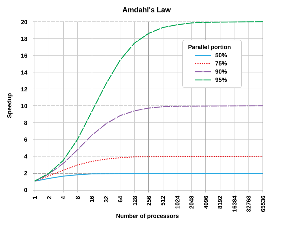
Real systems often do worse than flatten. Workers also pay for agreeing with each other about the shared data. On one machine, each CPU core keeps its own cached copy of data it uses, so when one worker changes the shared counter the other cores' copies have to be updated or thrown away (chapter 02 covers these caches). Across machines, servers send each other messages to stay in sync. Either way, every worker may need to hear from every other, and the number of pairs grows with the square of the number of workers: 4 workers make 6 pairs, 16 make 120. Neil Gunther's Universal Scalability Law (USL) puts both costs into one formula:
C(N) = N / (1 + α(N−1) + βN(N−1))C(N) is the throughput with N workers, measured as a multiple of what one worker achieves. α is contention, the serialised fraction. β is coherency, the cost of workers having to agree with each other. With β = 0 the formula is exactly Amdahl's law.
To see the shape, take made-up values α = 0.05 and β = 0.002:
Look at the solid curve. It follows Amdahl's at first, falls behind it as N grows, and reaches its top at 7.4 times one worker around 22 workers, which is √((1−α)/β). Past that point, every worker you add lowers the total. At 64 workers the system delivers 5.2 times one worker, less than it did with 8.
?How can adding capacity remove throughput?
Through the β term, which Amdahl's law leaves out. It's quadratic in N, because every worker may need to communicate with every other. Past some size that crosstalk grows faster than the capacity you added, and the curve turns downward.
5.2Fitting the USL to a real service
The values above were made up to show the shape. For a real service, Gunther's method is to measure throughput at several worker counts, choose the α and β that make the formula pass closest to the measurements, and use the formula to predict worker counts you haven't tried. The fit is useful because each coefficient points at a different cause:
| Fitted result | What it's telling you | Where to look |
|---|---|---|
Large α | A serialised section limits you | Find the lock |
Non-zero β | Workers are talking to each other too much | Coordination between workers; past the peak, each extra worker lowers throughput |
| Both near zero | Scaling is close to linear | Keep adding workers |
The USL predicts how much work the whole system gets done. It says nothing about what an individual request goes through while the workers fight over a lock, and that turns out to be the more dangerous part.
06What contention does to the tail
6.1The median improves while the p99 gets eleven times worse
Waiting is uneven. Most requests are lucky, and a few get stuck behind a burst, so the slow end of the latency distribution moves first. That slow end is called the tail. To describe it we use percentiles, the same idea as the p99 from section 1: the median (p50) is the latency half the requests beat, p90 and p99 are the latencies that 90 and 99 requests in 100 beat, p99.9 is the latency that 999 in 1,000 beat, and max is the slowest one.
A lock is the one-worker server from section 1 in another form: one thread at a time gets through, and the rest wait in line. Here is a lock under contention, with many threads wanting it at once. In this test, N threads each take the same lock, add one to a shared counter, and release the lock again, 100,000 times per thread, and every single acquisition is timed on its own, on a 10-core laptop. The timer only ticks about every 42 ns, which is slower than taking a lock nobody else wants, so at one thread most acquisitions read as 0 ns and the p50 is 0.
| threads | p50 | p90 | p99 | p99.9 | max |
|---|---|---|---|---|---|
| 1 | 0 ns | 42 ns | 42 ns | 42 ns | 334 ns |
| 2 | 83 ns | 84 ns | 125 ns | 1.6 µs | 20.7 µs |
| 4 | 208 ns | 209 ns | 2.1 µs | 30.9 µs | 854 µs |
| 8 | 42 ns | 167 ns | 23.9 µs | 56.5 µs | 157 µs |
Compare the 8-thread row against the 4-thread row. The median got five times better, 208 ns down to 42 ns. The p99 got eleven times worse, 2.1 µs up to 23.9 µs. Watching only the median, you'd have shipped the move from four threads to eight as an improvement.
Worst of all is the 4-thread max: 854 microseconds, about four thousand times the median, to acquire a lock that guards a single counter increment.
The plot below draws the same rows with latency on a log axis, where each step up the axis is ten times the one below. A steep line means latency multiplies quickly as you move from common requests towards rare ones.
Adding threads made the typical acquisition faster and the rare one far slower. To see how one lock can do both at once, we need to follow the threads.
6.2A lock convoy, step by step
?How can the median improve while the tail gets worse?
Because under contention the latencies split into two crowds, and the reason lies in what a thread does while it waits. When a thread finds the lock taken, it can park: it asks the kernel, the core of the operating system, to put it to sleep until the lock is free, so it uses no CPU while it waits. A parked thread can't run again until the holder releases the lock and the scheduler, the part of the kernel that decides which thread runs on each CPU (chapter 06), wakes it up. Waking takes time, and the holder doesn't wait for it. Here is what that does to eight threads sharing one lock.
A line of sleeping threads stuck behind one lock is called a convoy, and chapter 13 shows how one forms from the lock's side. In this test the convoy has a twist: the lock doesn't hand itself to the sleepers in turn, so the thread that's already awake keeps winning it. The holder's long batch makes most acquisitions cheap, which pulls the median down, and the threads that sat out the batch pay for all of it, which pushes the p99 up.
6.3The formula says nothing about fairness
Go back to the formula from section 3. 1/(1−ρ) predicts the mean wait, and it has nothing to say about who waits, which is the question of fairness: whether waiting is shared out evenly or piled onto a few. In a convoy some requests are served in a fast batch while others wait far longer, and that split and an even one can have the same mean. The formula can't tell them apart, so only the percentiles show you which one you have.
Everything so far happened inside one server. A user's request, though, often touches many servers at once, and the tail behaves differently there.
07Fan-out
7.1The slowest of a hundred
Many pages are built by asking a lot of other services, called backends, for pieces of the answer. A search page, for instance, might ask a hundred servers that each hold one slice of the index. The page can't be finished until every piece is back, so it waits for the slowest. When a request waits on N backends this way, that is called fan-out, and the page doesn't get a backend's p99. It gets the slowest of N draws.
A page calls 100 backends in parallel. Each backend is slow on 1% of calls, independently of the others. About what share of pages hit at least one slow call?
If each backend is slow on just 1% of calls, the chance that a page is fast is the chance that every call is fast:
| One backend's p99 | 1 call in 100 is slow | 0.99 fast |
| Fan out to 10 | 0.99¹⁰ | 90% all-fast |
| Fan out to 100 | 0.99¹⁰⁰ | 37% all-fast |
| Fan out to 500 | 0.99⁵⁰⁰ | 0.7% all-fast |
| at 100 backends, requests hitting someone's p99 | 63% | |
A backend's rare bad case becomes the user's normal case. That's the argument of Dean and Barroso's The Tail at Scale. It also changes what a good backend has to be: for the page's own p99 to be fast, 99 pages in 100 must have all hundred calls fast, which needs each backend to be fast on 99.99% of calls, not just 99%. We can check the 63% by letting a script roll the dice.
The script builds 100,000 pages for each fan-out size. For every page it makes fanout calls, each of which is slow with probability 0.01, and counts the pages where at least one call was slow. rng.random() < slow_chance is true 1% of the time, any(…) is true if any call in the page was slow, and the fixed seed makes the output repeatable.
import random

rng = random.Random(7)

def share_hitting_a_slow_call(fanout, pages=100_000, slow_chance=0.01):
    hit = 0
    for _ in range(pages):
        if any(rng.random() < slow_chance for _ in range(fanout)):
            hit += 1
    return hit / pages

print(f"{'backends per page':>17}  {'pages with a slow call':>22}")
for n in (1, 10, 100, 500):
print(f"{n:>17} {share_hitting_a_slow_call(n):>22.1%}")backends per page pages with a slow call
1 1.0%
10 9.6%
100 63.4%
500 99.4%The simulated shares match the arithmetic: 9.6% against 10%, 63.4% against 63%, and at 500 backends almost every page (about 99%) sees a slow call. Every backend in every row is slow on the same 1% of calls, so the whole climb comes from the number of draws per page.
7.2Hedged requests
Since the cause is the number of draws, large fan-out systems attack it with hedged requests. A hedge duplicates a request that's running late and takes whichever answer comes first. It needs a second replica of the backend, another copy that can answer the same question. Here is one call of a fan-out going wrong, then rescued:
?Why does a hedge cost so little?
Because it only fires for requests already slower than p95. Duplicating at p95 costs maybe 5% extra load, and it can cut the p99 dramatically.
All of these numbers depend on the latencies you collected being right, and very often they aren't.
08Measuring latency without fooling yourself
8.1Coordinated omission
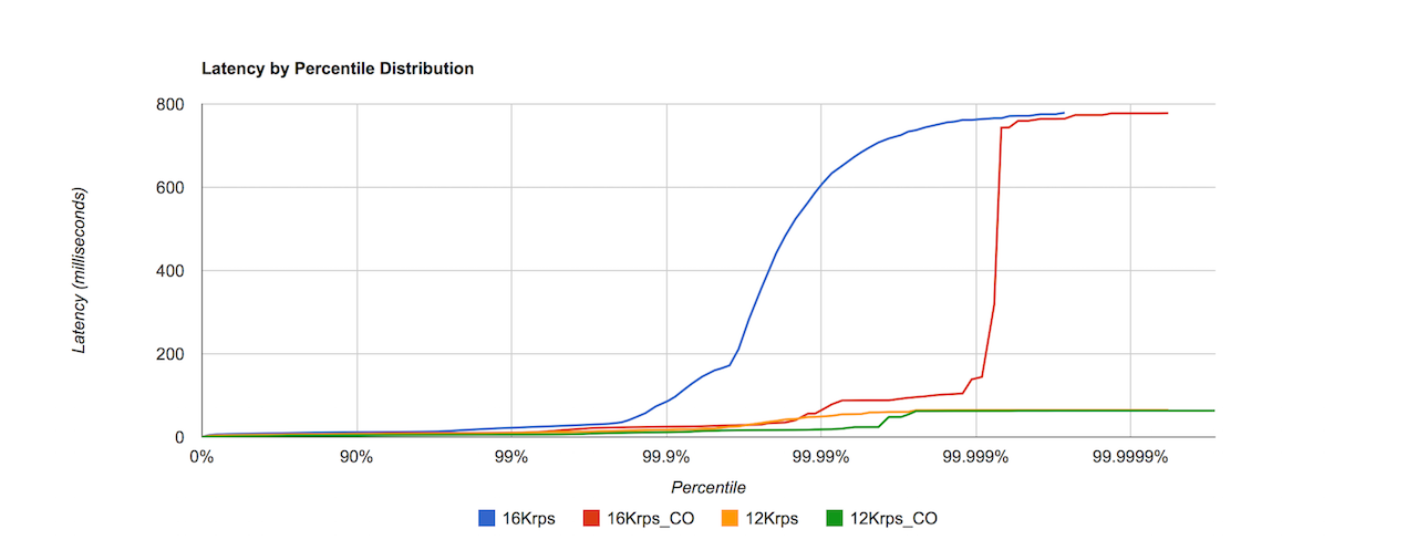
Latency numbers come from a load generator, a program that sends test requests to a service and records how long each one took. It keeps the times in a histogram, a table of how many requests fell into each latency range, and the report's p50 and p99 are read from it. Now take a one-worker service like the one from section 1, this time with requests that need 0.5 ms of work each, so that 1,000 requests a second keep it half busy (ρ = 0.5). Point a load generator at it that's meant to send those 1,000 requests a second, and make the service freeze for one second in the middle of the test. Suppose the generator is written the usual way: send a request, wait for the response, send the next.
Gil Tene named this coordinated omission: the generator and the service coordinate, because the generator stops sending exactly when the service stalls, so the slow requests that should have existed are never created. It's probably the most common reason a latency number is wrong. The queueing arithmetic from sections 3 and 4 still holds, but it can only be as good as the latencies you feed into it.
The script below plays both generators against the same freeze. There are 10,000 requests, one due every millisecond for ten seconds, each needing 0.5 ms of work, and between 5,000 ms and 6,000 ms the service can't start anything. It reuses the trick from the first simulation: start = max(sent, server_free) makes a request wait until the service is free. With wait_for_reply set, sent = max(due, prev_done) holds each request back until the previous reply has arrived, and latency is measured from sent. Without it, every request goes out on time and latency is measured from due.
def run(wait_for_reply, rps=1000, seconds=10, work_ms=0.5, stall_ms=(5000, 6000)):
    gap = 1000 / rps                       # one request is due every 1 ms
    server_free = 0.0                      # when the service can take the next request
    prev_done = 0.0
    lat = []
    for i in range(rps * seconds):
        due = i * gap                      # the intended send time
        sent = max(due, prev_done) if wait_for_reply else due
        start = max(sent, server_free)
        if stall_ms[0] <= start < stall_ms[1]:
            start = stall_ms[1]            # the service freezes until the stall ends
        done = start + work_ms
        server_free = prev_done = done
        lat.append(done - (sent if wait_for_reply else due))
    lat.sort()
    pick = lambda q: lat[int(q * len(lat))]
    return pick(0.50), pick(0.99), lat[-1]

print(f"{'generator':<28}{'p50':>9}{'p99':>10}{'max':>10}")
for name, wait in (("waits for each reply", True), ("measures from due time", False)):
    p50, p99, mx = run(wait)
print(f"{name:<28}{p50:>6.1f} ms{p99:>7.1f} ms{mx:>7.1f} ms")generator p50 p99 max
waits for each reply 0.5 ms 0.5 ms 1000.5 ms
measures from due time 0.5 ms 951.0 ms 1000.5 msBoth generators saw the same service and the same freeze, and the median is 0.5 ms for both. The max column shows that both noticed the freeze: a request did take about a second. But the first generator's p99 is 0.5 ms, because that one slow sample is lost among 9,999 fast ones. The second reports 951 ms, because its slowest 1%, the top hundred of the roughly 2,000 late requests from the last frame of the scene, all waited between about 950 and 1,000 ms.
?Why is it worse than ordinary noise?
Because noise scatters errors in both directions and averages out, while this error always points the same way. The generator drops samples exactly when the service is at its worst, so it erases the very tail you were trying to measure.
8.2Measuring against an intended schedule
The fix is the one in the second row of the output: measure from the time each request should have been sent. If you meant to send at 1,000 requests per second and a request that should have gone at t=5.000 s went at t=5.400 s, it has already accrued 400 ms before the service saw it. The tools below are load generators, and some of them do this for you. HdrHistogram is a library for recording latencies at constant cost across a huge range of values, and the honest tools use it underneath.
| Tool | Corrects for coordinated omission? |
|---|---|
wrk2 (use -R) | Yes: fixed intended rate |
oha | Only with a fixed rate (-q) and --latency-correction |
| Anything built on HdrHistogram with rate correction | Yes |
ab | No |
| A naive request loop | No |
8.3Percentiles don't average
A last trap is in how numbers get combined. Averaging the p99s from ten app servers doesn't give you the fleet's p99. One reason is that an average gives a server that handled ten requests the same weight as one that handled a million. Another is that a percentile depends on the shape of the whole distribution: if one server out of ten is stuck in a convoy, the slowest 1% of all requests may come almost entirely from it, and averaging its p99 with nine healthy ones hides that. Merge the underlying histograms and take the p99 of the combined distribution.
We now have a full toolbox: the utilisation curve, Little's Law, the USL, the tail arithmetic of fan-out, and a way to measure honestly. What's left is how to use them on a real service.
09Applying it to your service
9.1Four checks, in order
Work these in order. Each one takes a minute and rules something out.
- Little's Law on your dashboard (section 4). Compute
L = λWfrom throughput and latency, and compare it against your thread pool or connection pool size. IfLis at the pool limit, the pool is your bottleneck. - Find your ρ (section 3). Take the utilisation of the resource requests are queueing for, which is often a pool, a lock or a disk rather than the CPU. If it's past 0.8, your latency is dominated by queueing, and adding headroom beats optimising.
- Fit the USL (section 5). Measure throughput at 1, 2, 4, 8 and 16 workers and fit
αandβ. A largeαmeans find the serialised section. A non-zeroβmeans your workers are talking to each other. - Check your load generator (section 8). Before trusting any of the above, confirm it corrects for coordinated omission. If it doesn't, your latency data is biased in the unsafe direction and everything else is built on it.
9.2Rules that hold up
- Keep shared resources below the knee. Past about 80% busy, the queue dominates latency (section 3).
- Judge a change by its p99 and p99.9 as well as its median. A convoy improves the median while the tail gets worse (section 6).
- Measure the utilisation of the resource that is queueing. CPU is often a different resource (section 3).
- Check the load generator before trusting a latency number (section 8).
- For fan-out, change the architecture. Hedge after p95, reduce the fan-out, or accept partial answers (section 7).
9.3What each fix buys
| Intervention | What it buys | Note |
|---|---|---|
| Reduce utilisation | The curve is superlinear, so past the knee headroom buys more than optimisation | 90% to 80% halves the time in the system |
| Shard the contended thing (split it into independent pieces, each with its own lock) | Removes the serialised section | Chapter 17 measures this at 16× |
| Shorten the critical section | Less time holding the lock | Move allocation, I/O and logging out |
| Hedge | Cuts p99 dramatically under fan-out | Costs maybe 5% extra load |
| Shed load (refuse some requests quickly) | Refusing 1% quickly beats serving 100% past the knee | People reach for this last and should reach for it third |
9.4Symptom, cause, fix
| Symptom | Likely cause | Fix |
|---|---|---|
| p99 grew tenfold, p50 flat, CPU unchanged | A convoy on a shared resource | Check off-CPU time and lock contention; shard or shorten the critical section |
| Handler optimisations don't move latency | L = λW is at the pool limit | Grow the pool, or cut W elsewhere |
| Latency climbs steeply above ~80% of a resource | Past the knee of 1/(1−ρ) | Add headroom, or shed load |
| Adding nodes or threads lowers throughput | The USL's β term: crosstalk | Reduce coordination between workers |
| Load test p99 looks great, users see stalls | Coordinated omission | Re-run with wrk2 -R or an HdrHistogram-based tool |
| Page latency far above any backend's p99 | Fan-out to many backends | Hedge at p95, reduce fan-out, accept partial answers |
10Summary
- Every shared resource is a queue: locks, pools, disks and event loops all follow the same arithmetic.
- Waiting comes from bursts. Three requests arriving together make the third wait two milliseconds for one millisecond of work, and quiet time afterwards doesn't undo it.
- Time in the system grows as
1/(1−ρ). Twice the work at 50% busy, ten times at 90%, twenty at 95%. - The model is optimistic. Bursty arrivals and long-tailed service make real queues worse than it predicts.
- Little's Law needs no assumptions.
L = λWfrom your dashboard tells you whether the pool is the bottleneck. - The USL's
βterm makes scaling turn downward, because crosstalk grows quadratically with workers. - Contention hits the tail first. In the lock test, going from four threads to eight made p50 five times better and p99 eleven times worse.
- A convoy splits the distribution, and a CPU profile can't see the threads that are waiting.
- Fan-out turns a backend's p99 into the user's normal case: 63% of requests at a hundred backends.
- Hedging at p95 costs about 5% extra load and can cut the p99 dramatically.
- Most load generators hide stalls. Measure against an intended schedule, and merge histograms instead of averaging percentiles.
11Build this
A tail-latency lab on your own laptop.
- Time 100,000 lock acquisitions per thread at 1, 2, 4 and 8 threads, and print p50, p90, p99, p99.9 and max. Check whether your machine shows the same split as section 6.1.
- Measure a toy service's throughput at 1, 2, 4, 8 and 16 workers and fit the USL's
αandβ. - Load-test it twice at a fixed rate, once with a closed loop that waits for each response and once with
wrk2 -R, while you inject a one-second pause. Compare the two p99s, as the two generators in section 8 did.
12Interview questions
beginnerWhat does Little's Law say and when does it apply?›
L = λW: items in the system equals arrival rate times time in the system. It applies to any stable queue with no assumptions about arrival or service distributions. That generality is what makes it useful: given any two of concurrency, throughput and latency you get the third.
In practice it's the fastest way to find out whether your connection pool is the bottleneck. Compute L from your dashboard and compare it to the pool size.
intermediateYour p50 is flat and p99 grew tenfold. CPU is unchanged. What's happening?›
Probably a convoy on a shared resource. Threads park behind a holder, one runs a long uninterrupted batch so its acquisitions are fast and the median looks fine, while parked threads wait far longer.
A test of one lock shows exactly this going from four threads to eight: p50 improved from 208 ns to 42 ns while p99 went from 2.1 µs to 23.9 µs. Look at off-CPU time and lock contention, not a CPU profile: a blocked thread burns no cycles and never appears in a flame graph.
intermediateWhy does 90% to 95% utilisation hurt so much more than 50% to 55%?›
Because time in the system scales as 1/(1−ρ), not linearly. At 50% it's about two service times, at 90% ten, at 95% twenty. The same five-point increase costs ten service times at the top and a fraction of one at the bottom.
Past the knee, headroom is worth more than optimisation, and the curve is an optimistic bound, since real traffic is burstier than Poisson.
deepWhat is coordinated omission and why does it matter?›
A load generator that waits for each response before sending the next stops generating load exactly when the system stalls. A one-second stall produces one slow sample instead of the thousand requests that should have arrived, so the tail is erased.
The bias is worst precisely when the system is worst. Fix it by measuring from the intended send time: a request meant to go at 1,000 rps that departs 400 ms late has already accrued 400 ms. Use wrk2 or anything built on HdrHistogram with rate correction, and with oha combine -q and --latency-correction.
deepYour service calls 100 backends per request, each with a 10 ms p99. What's your p99?›
Far worse than 10 ms. The probability that all hundred return fast is 0.99¹⁰⁰ ≈ 0.37, so about 63% of requests wait on at least one backend's p99. Your p99 is set by the slowest of a hundred draws, which works out to each backend's 99.99th percentile.
The fixes are in the architecture: hedge after p95, reduce fan-out, or make the call tolerant of a partial answer. That's the core argument of The Tail at Scale.
13Go deeper
Is it valid to average the p99s from your ten app servers?›
No. Percentiles don't average. Merge the underlying histograms and take the p99 of the combined distribution.
Load test shows p99 of 3 ms. The service froze for 2 seconds during the run. Explain.›
Coordinated omission. Your generator stopped sending during the freeze, so the stall contributed a handful of samples instead of thousands.
USL predicts throughput decreasing past some node count. Which term, and why?›
The β coherency term. It's quadratic in N because every node may need to communicate with every other, so crosstalk eventually grows faster than the capacity you added.
Adding threads improved your median. Ship it?›
Not without checking the tail. A convoy improves the median by batching while making p99 dramatically worse. That's the 4-to-8-thread row.
Google's account of why tail latency dominates at scale, and what they did: hedged requests, tied requests, micro-partitioning, selective replication.
The talk that named coordinated omission, including a demonstration where a system that stalled for 100 seconds reports a p99 of a few milliseconds.
Where the USL comes from, including how to fit α and β against measurements you already have.
Constant-cost recording across a huge dynamic range. What every honest load generator uses underneath.
Gil Tene's fork of wrk with a fixed intended rate and correction for
coordinated omission. Use -R.
The USE method and off-CPU analysis. The best single treatment of finding latency a CPU profile cannot see.
14Related chapters
How a mutex spins, parks and wakes: the mechanics behind the convoy in section 6. Chapter 13.
Threads, async and goroutines, and why every one of them needs a bound. Chapter 15.
Sharding the contended thing, measured at 16×. Chapter 17.
How the scheduler decides which thread runs next, which is what wakes the threads parked in a convoy. Chapter 06.