Ana is sitting in a café in Lisbon with a coffee and a plan. She opens the map on her phone, and the streets around her appear almost before her thumb has left the icon. She drags the map north-east, past Madrid and the Pyrenees, and new streets, rivers and town names keep sliding into view as fast as she can drag. She types "Berl", picks Berlin from the suggestions, and taps Directions. Within about a second a blue line runs from her café, across Spain, France and Germany, to the Brandenburg Gate, with an arrival time attached. A small red stretch near Heidelberg shows a jam that's already slowing people down.
Each of those moments hides a problem that isn't obvious from the café. The map Ana drags across covers the whole planet, at every level of detail from continents down to footpaths, and something has to decide which small piece of it to send to her phone, and keep that fast for two billion people. Behind the blue line is a shortest path through a graph of tens of millions of junctions, and the textbook algorithm for it takes seconds, far too long for a tap. And the arrival time depends on roads Ana won't reach for twenty hours, and on a jam near Heidelberg that might have cleared by the time she gets there.
In this case study we'll design the system that answers Ana, the way an engineer would: start with the most obvious design, find where it breaks, and fix it. The question we'll keep coming back to is this: how does a map draw any part of the world instantly, and find the fastest route across a continent, with live traffic, in about a second? Chapter 50 already covered how Uber indexes moving cars with geohashes and hexagons, and how a road network becomes a graph, so we won't repeat those. We'll go elsewhere: from map tiles and their maths, through the data structure that makes continental routing fast, to where traffic data comes from and how a neural network turns it into an arrival time.
01What we're building, and how big
1.1What it has to do
Strip away Street View, reviews and the rest, and the core of a map service that gets Ana to Berlin comes down to this:
- Draw the map for any place on Earth at any level of detail, and keep up while the user drags and pinches.
- Find places: turn "Berl" into Berlin, and a typed address into a point on the map.
- Find a route between two points, by road, over any distance.
- Predict the arrival time, the ETA (estimated time of arrival), along that route, including the traffic the driver will meet on the way.
- Show live traffic on the map, and reroute when it changes.
And the qualities it needs:
- Fast to draw: dragging the map should feel like moving paper, so new parts of the map have to arrive in tens of milliseconds.
- Fast to route: a route across a continent in well under a second, for any pair of points, because nobody can precompute every pair.
- Fresh: traffic that's ten minutes stale is wrong exactly when it matters most.
- Accurate: an arrival time that's twenty minutes off is worse than none, because people plan around it.
Notice that the map and the route are very different problems. Drawing the map is a question of serving the same data to huge numbers of people, so it's about caching. Routing is a question of computing a different answer for every request, so it's about algorithms. Sections 2 to 4 deal with the first problem, and sections 5 to 9 with the second.
1.2How big is it?
Alphabet said in October 2024 that Google Maps had passed two billion monthly users. Back in September 2020, when DeepMind and Google described their work on arrival times, Google Maps already served more than a billion people, and its predicted arrival times were "consistently accurate for over 97% of trips".
Google doesn't publish how many map requests it serves, but OpenStreetMap, the open, volunteer-built map of the world, does publish numbers for its own tile service, and it gives a sense of scale. In July 2025 its servers answered 92 billion requests for map pieces, about 36,800 a second on average, each about 18 KB, which adds up to 1.26 petabytes in a month. That's one free community map. Google's traffic is probably far larger.
Road networks are big as well. A standard research benchmark for routing is the road network of Western Europe, with 18 million junctions and 42.5 million one-way road segments. Ana's trip crosses a good part of it.
Suppose we cut the world map into small square pictures, 256 pixels on a side, at 19 levels of detail, where each level has four times as many pictures as the one above (1, 4, 16, …). How many pictures is that, and if each one is about 18 KB, how much storage?
02Drawing the map: tiles
2.1Version 1: draw a picture for every request
The obvious design is a map server that draws pictures. Ana's phone sends the latitude and longitude of the corners of her screen and its size in pixels. It queries a database of roads, rivers and labels for everything inside that box, draws them into an image, and sends it back. When she drags the map, the phone asks for a new picture.
It works for one user and breaks for two billion, for one reason: no two requests are the same. Ana's screen box is a little different from everyone else's, and different again every time she drags, so nothing the server draws can be reused. Every pixel on every screen is drawn fresh, which means a database query and a rendering job for every drag, and a wait while it happens. Caching, the usual answer to "lots of people want the same thing", can't help when nobody asks for the same thing twice.
The fix is to make everyone ask for the same things. Cut the map into a fixed grid of small squares, the same grid for every user, and have the phone ask for the squares that overlap its screen. Ana's screen might need fifteen of them; the person in the next café needs fourteen of the same fifteen. Each square, once drawn, can be stored and handed to everyone who asks for it. Those squares are called tiles, and the rest of this section is about how to cut them.
2.2Flattening the Earth: Web Mercator
Before we can cut the map into squares we need a flat map to cut, and the Earth is round. Turning positions on a sphere into positions on a flat plane is called a projection, and every projection distorts something: areas, distances, angles or shapes. Web maps chose the Mercator projection, which Gerardus Mercator designed for sailors in 1569.
Mercator has two properties a street map needs. North is always straight up, so a street grid that runs north-south on the ground runs up-down on the screen. And it preserves angles locally: a crossroads where two streets meet at right angles still looks like a right angle, anywhere on Earth. A map that bent the corners of Berlin's streets would be useless for finding your way.
Size is the price. Mercator stretches everything more and more as you move away from the equator. That's why Greenland looks as big as Africa on most web maps, when Africa is about fourteen times larger.
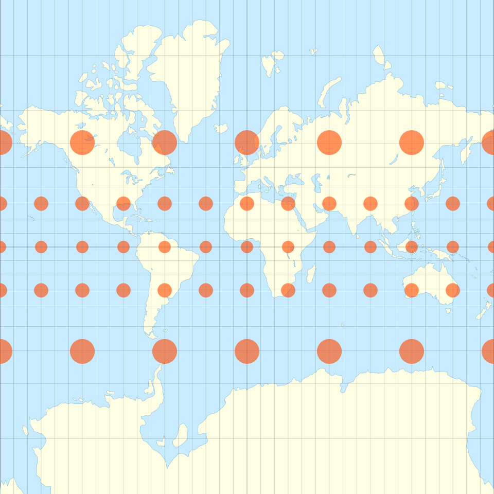
Mercator also stretches the poles to infinity, so a web map has to stop somewhere. The version used by Google Maps since 2005, and now by almost every web map, is called Web Mercator. It cuts the world off at about 85.05° north and south, a latitude chosen for one reason: it makes the whole flattened world exactly square. (The exact limit is the arctangent of sinh(π), 85.0511°.) A square world is what makes the grid of tiles simple.
2.3The tile pyramid: z, x and y
Now cut the square. At the coarsest level of detail, the whole world is one square picture, 256 pixels on a side. That's zoom level 0. At zoom level 1 the world is drawn twice as wide and cut into a 2 × 2 grid of 256-pixel squares, so 4 tiles. At zoom 2 it's 4 × 4, 16 tiles, and so on: each level doubles the width and height, so every tile splits into four tiles at the next level. At zoom z the world is 2z tiles across and 4z tiles in all. Stacked up, the levels form a tile pyramid.
Every tile is named by three numbers: its zoom z, its column x counted from the left (from 180° west), and its row y counted from the top (from 85.05° north). That's the whole addressing scheme, and it's why tile URLs look like /15/15552/12555.png.
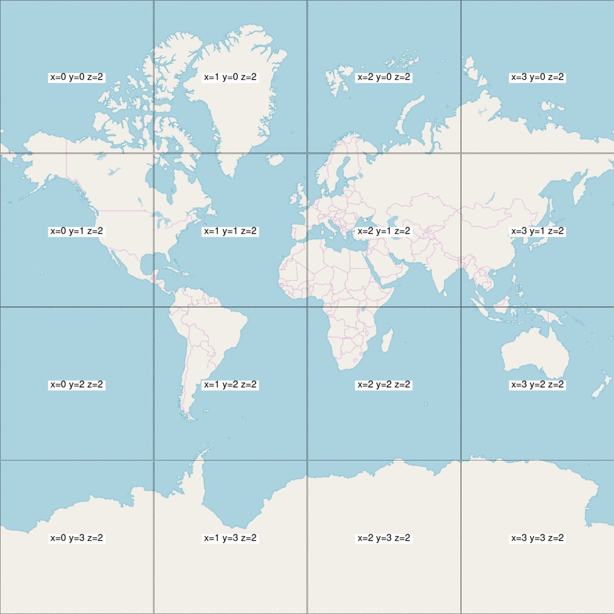
Turning a latitude and longitude into a tile is two formulas. Longitude maps to x in a straight line, since Mercator spaces meridians evenly. Latitude maps to y through the Mercator stretch, which grows with latitude. Both formulas are on the OpenStreetMap wiki, and this program uses them to find which tile holds Lisbon and which holds Berlin at a few zoom levels. math.asinh(math.tan(lat)) is the Mercator stretch for a latitude in radians, and int() rounds down to a whole tile number.
import math

def tile(lat, lon, z):
    n = 2 ** z                                   # tiles across at zoom z
    x = (lon + 180) / 360 * n
    lat_r = math.radians(lat)
    y = (1 - math.asinh(math.tan(lat_r)) / math.pi) / 2 * n
    return int(x), int(y)

places = {"Lisbon": (38.7223, -9.1393), "Berlin": (52.5200, 13.4050)}
for z in (0, 1, 5, 10, 15):
    row = "  ".join(f"{name} {tile(lat, lon, z)}" for name, (lat, lon) in places.items())
    print(f"z={z:<2} {4 ** z:>14,} tiles  {row}")

# how much ground one 256-pixel tile covers at Lisbon's latitude
for z in (5, 10, 15):
    m_per_px = 156543.03 * math.cos(math.radians(38.7223)) / 2 ** z
print(f"z={z:<2} one tile is about {m_per_px * 256 / 1000:,.1f} km wide in Lisbon")z=0 1 tiles Lisbon (0, 0) Berlin (0, 0)
z=1 4 tiles Lisbon (0, 0) Berlin (1, 0)
z=5 1,024 tiles Lisbon (15, 12) Berlin (17, 10)
z=10 1,048,576 tiles Lisbon (486, 392) Berlin (550, 335)
z=15 1,073,741,824 tiles Lisbon (15552, 12555) Berlin (17604, 10746)
z=5 one tile is about 977.1 km wide in Lisbon
z=10 one tile is about 30.5 km wide in Lisbon
z=15 one tile is about 1.0 km wide in LisbonRead the output from the top. At zoom 0, Lisbon and Berlin are in the same tile, because there's only one. At zoom 1 they split: Lisbon is just west of the Greenwich meridian, in the left column, and Berlin is in the right one. By zoom 15 there are over a billion tiles, and one tile covers about a kilometre of Lisbon, roughly a neighbourhood with its street names readable. Where does 156,543 come from? It's the Earth's circumference at the equator, about 40,075 km, divided by the 256 pixels of the zoom-0 tile: the metres that one pixel covers at zoom 0. Multiplying by the cosine of the latitude corrects for Mercator's stretch, so a tile in Lisbon covers less ground than a tile of the same zoom on the equator.
Tile numbers also say how tiles relate across zoom levels. Lisbon's zoom-10 tile is (486, 392). Its parent at zoom 9 is (243, 196), half of each number rounded down, and its four children at zoom 11 are (972, 784), (973, 784), (972, 785) and (973, 785). Like an H3 or S2 cell ID from chapter 50, a tile address is a path down a hierarchy, and moving up or down is arithmetic.
Ana's screen shows a 3 × 5 block of tiles at zoom 12. She pinches to zoom in by exactly one level, keeping the centre of the screen fixed. Roughly how many new tiles does her phone need?
2.4Serving tiles: render once, cache everywhere
Tiles fix version 1's problem: requests now repeat. Everyone looking at central Lisbon at zoom 15 asks for the same few tiles, by the same URLs, so a tile drawn once can be stored and served to all of them. The next question is when to draw each tile, and where to keep it.
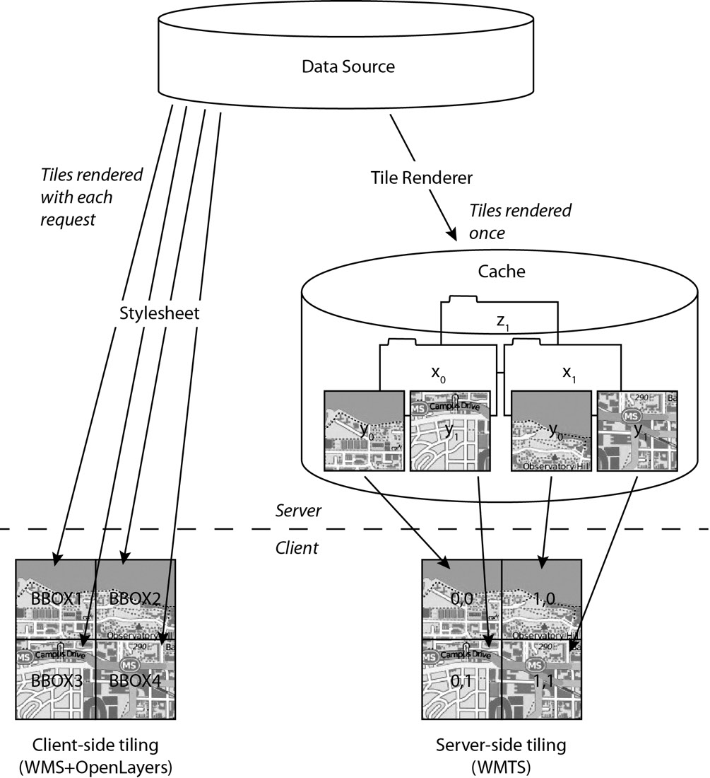
Back in the estimate in section 1.2, we saw that pre-rendering the whole pyramid to zoom 18 would mean about 92 billion tiles, most of which nobody will ever look at. So the practical answer is a mix: pre-render the levels that cover the whole world in few tiles (up to zoom 10 or so is about 1.4 million tiles), and draw deeper tiles on demand, the first time someone asks for one, then keep the result.
OpenStreetMap's tile servers show the details of drawing on demand. They don't render one 256-pixel tile at a time. They render a metatile, a block of 8 × 8 tiles, 2048 pixels square, in one go, and cut it up afterwards. That has two benefits. Starting a render and fetching the map data is the expensive part, so doing it once for 64 tiles is much cheaper than 64 times. And labels come out better, because a street name or a long road's label can be placed once across the big area without being chopped at every small tile's edge.
In front of the renderers sits a content delivery network (CDN): a fleet of cache servers spread around the world, each keeping copies of popular files close to the people asking for them (chapter 35 covers how they work). A request for a tile goes to the nearest CDN server first, and only if that server doesn't have the tile does it travel on to a render server. For OpenStreetMap, that CDN is Fastly, and in August 2025 its operations team reported that about 97% of tile bytes were served straight from the CDN's caches, and the render servers' own caches answered over 95% of what got through.
?When the map changes, how do cached tiles find out?
Slowly, by design. Each tile is sent with HTTP caching headers that say how long it can be kept, and every cache along the way, phone, CDN and origin store, keeps it until then. OpenStreetMap's tile policy asks apps that can't read the headers to keep tiles for at least seven days. When a mapper fixes a road, the tiles covering it are marked stale at the origin and re-rendered, but copies already in caches live on until they expire. Since July 2025, OpenStreetMap's CDN has honoured the "this tile has changed" signal only for requests from openstreetmap.org itself, where mappers want to see their edits; other apps get the older cached tile, which spares the renderers. A street map that's a few days behind is fine for almost everyone. Traffic, which changes by the minute, can't work like this, which is one reason it's handled separately, in section 7.
Render every tile in advance, or when it's first asked for?
- Every request is a file read
- No render load at request time
- About 92 billion tiles to zoom 18, mostly ocean nobody visits
- Re-rendering after every edit is enormous
- Work is spent only on tiles people look at
- Popular tiles are served from caches near the user
- The first viewer of a rare tile waits for a render
- Stale tiles linger in caches after edits
Popularity is so uneven that on-demand rendering costs little: a tile is drawn once and then read thousands or millions of times from caches. OpenStreetMap does this, with the low zoom levels kept warm because everyone passes through them. How Google renders and stores its tiles is unpublished, but the shape of the problem, a fixed grid of immutable named pieces with very skewed popularity, is the textbook case for a CDN.
03Pictures or blueprints: raster and vector tiles
3.1What's wrong with pictures
So far our tiles are pictures, grids of coloured pixels; these are called raster tiles. They're simple and every browser can show them, but they have three problems, and the Predict in section 2.3 already hinted at the first. A picture drawn for zoom 15 can't be redrawn for zoom 15.5; stretched, its roads and text blur. So the map can only sit at whole zoom levels, and every zoom step means downloading a fresh set of tiles. Second, a picture is drawn north-up with labels baked in, so if Ana rotates the map to face the way she's driving, every street name rotates with it and ends up upside down. Third, every style is a separate set of pictures: day, night, satellite with roads on top, each one rendered and stored again.
Google described all three problems in December 2010, when it switched its Android app away from pictures. The old app downloaded the map as 256 × 256 image tiles with "roads, labels and other features baked right in", and the post noted that it took "more than 360 billion tiles to cover the whole world at 20 zoom levels".
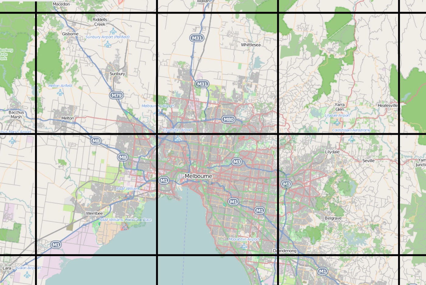
Google's fix was to send the data instead of the drawing. A vector tile covers the same z/x/y square as a raster tile, but instead of pixels it holds the geometry inside the square, the lines of roads, the outlines of buildings and parks, the points of shops, each tagged with what it is ("motorway", "name: Rua Augusta"). Ana's phone draws the picture itself, at whatever zoom, angle and style it wants. Google called vector tiles "the blueprints needed to draw a map, instead of static map images", and said that because one vector tile can be drawn across several zoom levels, viewing the map across all zoom levels needed more than 100 times less data than before.
3.2Inside a vector tile
Google's own vector format is unpublished, but the open format most of the industry uses is documented in detail. The Mapbox Vector Tile specification (version 2.1, 2016) is used by Mapbox, by OpenStreetMap-based maps and by many others, and it shows how small a tile can be made.
A vector tile is a Protocol Buffers message, Google's compact binary encoding for structured data. Inside are layers, such as "roads", "buildings" and "water", and each layer holds features: one road, one building. Coordinates inside a tile are small integers on the tile's own grid, typically 0 to 4,095 across (the layer's extent), with the origin at the top-left corner. Using the tile's own grid means a coordinate never needs more than 12 bits, however far the tile is from Greenwich.
A feature's shape is a list of drawing commands, as if guiding a pen. There are three: MoveTo (lift the pen and move), LineTo (draw a line) and ClosePath (close a polygon). Each command is one integer that packs the command's ID in its low 3 bits and how many times to repeat it in the rest: (id & 0x7) | (count << 3). After it come the coordinates, and each one is stored as the difference from the previous point, since neighbouring points along a road are close together and differences are small. Differences can be negative, so they go through zigzag encoding, which maps 0, −1, 1, −2, 2 to 0, 1, 2, 3, 4, keeping small numbers small whatever their sign.
Here's a short road that starts at (2, 2), runs down to (2, 10) and turns right to (10, 10):
The 9 is MoveTo (ID 1) with a count of 1: 1 | (1 << 3) = 9. And 18 is LineTo (ID 2) with a count of 2: 2 | (2 << 3) = 18. A coordinate of +2 zigzags to 4 and +8 to 16. Protocol Buffers then stores each of these small integers in a single byte, so the whole road takes eight bytes. Tags are squeezed the same way: each layer keeps one table of keys ("highway", "name") and one of values ("motorway", "Rua Augusta"), and a feature's tags are pairs of indexes into those tables, so the string "motorway" is stored once per tile, not once per road.
Should the server send pictures or geometry?
- Works on any client, even the oldest browser
- The client does no drawing work
- Style is guaranteed identical everywhere
- Whole zoom levels only; blurry in between
- Labels can't rotate with the map
- Every style is a separate set of images
- Smooth zoom, tilt and rotation
- One tile serves several zoom levels
- Styles (night, satellite overlay) cost nothing extra to serve
- Needs a capable client and a rendering engine on every platform
- Harder to guarantee identical results everywhere
Google moved its Android app to vector tiles in December 2010, once phone hardware could draw a map smoothly, and the 3D buildings, rotation and offline maps that followed all depend on it. Raster tiles are far from dead: OpenStreetMap's standard map layer, the one with 92 billion requests a month, was still served as raster tiles in 2025, because they work everywhere and any website can embed them with a few lines of code. Many systems serve both, generating raster tiles from the same vector data for old clients.
With the map on Ana's screen, she types "Berl". That's the next thing the system has to answer.
04Finding Berlin: search and geocoding
4.1From text to a point
Before the system can route to Berlin, it has to turn the letters Ana typed into a point on the map. Turning a name or an address into coordinates is called geocoding, and turning coordinates back into an address, as when Ana long-presses a spot and the map shows "Rua Augusta 24", is reverse geocoding. This chapter treats search briefly, since its machinery is closer to a search engine than to a map, but two parts of it matter for our design.
The first is that suggestions appear while Ana types. After "B", "Be", "Ber", "Berl" the list updates each time, so the system must find every place whose name starts with the letters so far, in a few milliseconds. That's a prefix lookup, and the classic structure for it is a trie, a tree where each edge is a letter and every name is a path from the root. All the names starting with "Berl" sit under one node, so finding them means walking four edges and reading off what's below. Production systems store each node's best few completions with it, so the walk ends with an answer ready.
Then there's ranking. "Berl" matches Berlin, but also Berlingen, Berlaar and hundreds of streets called Berliner Straße. Which comes first depends on how important each place is (a capital city outranks a village) and how close it is to where the user is looking: if Ana's map were showing Hamburg, the nearby Berliner Tor station would probably win. Google's ranking is unpublished. OpenStreetMap's open-source geocoder, Nominatim, built on PostgreSQL and its geographic extension PostGIS, breaks ties between equally good matches with an importance score for each place, derived mainly from how highly the place's Wikipedia page ranks.
Reverse geocoding is a spatial lookup: find the address points, streets and areas nearest to a coordinate. That's the same "what's near this point" question chapter 50 answered with geohashes, S2 cells and R-trees, so we'll leave it there.
Ana picks Berlin and taps Directions. Now the system has two points, one in Lisbon and one in Berlin, and has to find the fastest road between them.
05Finding the route: why the textbook algorithm is too slow
5.1Dijkstra across a continent
Chapter 50 showed how a road network becomes a graph: junctions are nodes, the stretches of road between them are edges, and each edge's weight is how long it takes to drive. The fastest route is the shortest path in that graph, and the textbook way to find it is Dijkstra's algorithm. It keeps a priority queue of nodes ordered by their distance from the start, repeatedly takes the closest node not yet finished, which is called settling it, and updates the distances of its neighbours. When it settles the destination, it has the answer.
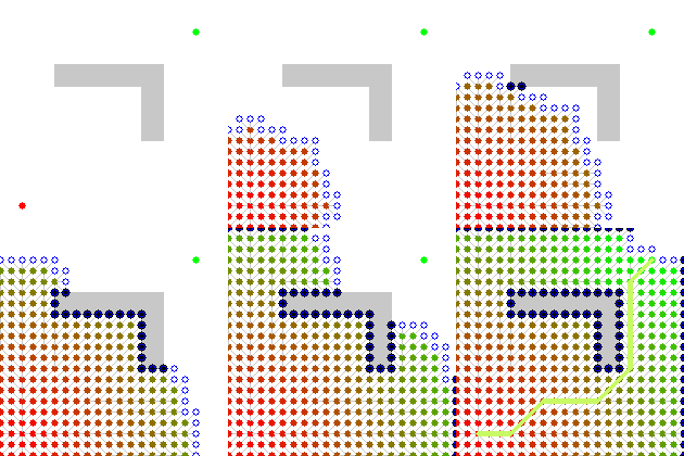
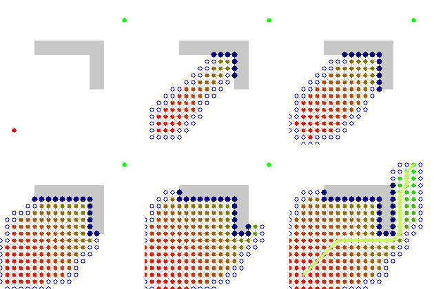
Look at the left animation. Dijkstra doesn't know where the goal is, so it grows a circle of settled nodes outward in every direction and stops only when the circle reaches the goal. For Ana's trip, that circle has a radius of a whole day's driving. It covers Portugal, Spain, France, much of Germany, and also, uselessly, Morocco's ferry ports and the Atlantic coast, because they're closer to Lisbon than Berlin is.
Routing researchers measured exactly this. In a 2015 survey of route-planning algorithms, Hannah Bast, Daniel Delling, Peter Sanders, Renato Werneck and their co-authors ran Dijkstra's algorithm on the Western Europe benchmark between random pairs of points. An average query settled 9.3 million of the 18 million nodes and took about 2.2 seconds on one core of a 2010-era server. Running two searches at once, one forward from the start and one backward from the destination, stopping when they meet, is called bidirectional search; it halves the work, to 4.9 million nodes and 1.2 seconds, because two circles of half the radius cover half the area of one big one.
Suppose two billion monthly users ask for, between them, a few hundred thousand routes a second at peak, and each takes 1.2 seconds of one CPU core. How many cores is that, and what's wrong besides the count?
5.2A*: pointing the search at Berlin
The obvious improvement is to stop exploring in directions that lead away from Berlin. A* (pronounced "A star") does this by changing the order in which nodes are settled: instead of a node's distance from the start, it uses that distance plus a guess of the distance still to go. Nodes in the direction of Berlin have small guesses and get settled first; nodes towards Morocco have large ones and wait. As long as the guess never overestimates the true remaining distance, A* still finds the shortest path. In the right-hand animation above, it seems to work well, and on that grid it does.
On a road network with travel times, though, A* disappoints, for a reason that's easy to miss. The guess has to be a lower bound on the remaining time. An obvious one is the straight-line distance to Berlin divided by the fastest speed anywhere in the network, since no route can beat that. But the fastest speed is a motorway speed, while most of the graph is slow streets, so the guess badly underestimates, and a guess that underestimates badly barely steers the search. According to the 2015 survey, with this bound "the performance gain is small or non-existent". Chapter 50 quoted Uber measuring about 120 ms for a city-scale A* query in 2015; at continental scale it's far worse.
A smarter guess helps a bit more. ALT (A*, landmarks and the triangle inequality) precomputes, for a handful of landmark nodes, the travel time from each landmark to every node, and uses those to compute much tighter lower bounds during a search. It's a real speed-up, but it still explores a corridor of the map, and corridors across a continent hold millions of nodes.
Ana's question needs something different in kind, and the hint is in how people plan long drives themselves. Nobody planning Lisbon to Berlin thinks about side streets in Bordeaux. You think: get from my street to the nearest motorway, stay on motorways for two thousand kilometres, get off near the destination. Long routes, almost whatever their start and end, funnel through a small network of important roads. The fastest routing algorithms are built on that observation, by doing a lot of work in advance.
06Contraction hierarchies
6.1Shortcuts around unimportant junctions
The algorithm we'll build was published in 2008 by Robert Geisberger, Peter Sanders, Dominik Schultes and Daniel Delling at the Karlsruhe Institute of Technology, under the title Contraction Hierarchies: Faster and Simpler Hierarchical Routing in Road Networks. It does its work in two phases: a slow preprocessing phase, run once whenever the map changes, and a fast query phase, run for every route.
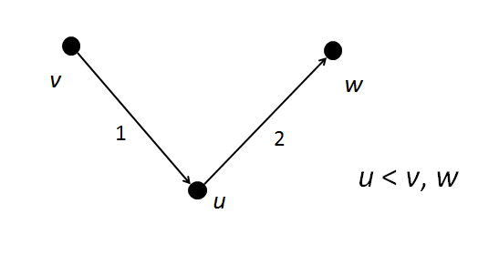
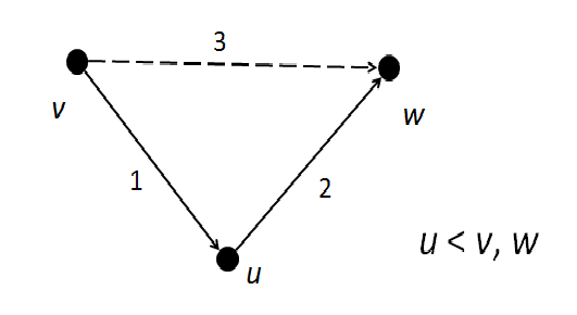
Preprocessing is built from one operation. Take a node, say a junction u on a quiet residential street, and remove it from the graph. Any shortest path that used to pass through u is now broken. To repair it, for each pair of u's neighbours v and w, check whether the path v → u → w was the only shortest way from v to w. If it was, add a new edge straight from v to w, with weight equal to the two edges it replaces. That new edge is called a shortcut, and removing a node while adding the shortcuts that preserve every shortest distance is called contracting it.
?How do we know whether v → u → w was the only shortest way?
By searching for another one. Before adding the shortcut, run a small Dijkstra search from v in the graph without u, limited to distances up to the cost of v → u → w. If it finds a path to w that's no longer, that path is called a witness, and the shortcut isn't needed, because the distance survives without it. In a grid of city streets there's often a witness one block over; on a lone country road between two villages there never is. Witness searches are what keep the number of shortcuts down, and they're most of the preprocessing time.
Preprocessing contracts every node in the graph, one at a time, in some order, from least important to most. Each node's position in that order is its rank. When it's done, we put back all the original nodes and edges and keep every shortcut, so the final graph is the original road network plus a large set of shortcuts, and every node has a rank. The shortcuts layered over the ranked nodes are the contraction hierarchy.
6.2Choosing the order
Order matters a great deal. Contract a motorway junction early and you'll need shortcuts between all its neighbours, for all the long routes that pass through it, and every later contraction inherits them. Contract a dead-end street first and it needs no shortcuts at all.
So preprocessing picks the order greedily, a node at a time. For every remaining node it computes a cost, and contracts the cheapest one next. The main part of the cost is the edge difference: how many shortcuts contracting the node would add, minus how many edges it would remove. A dead end removes one edge and adds nothing, so its edge difference is −1, and it goes early. A junction where four busy roads meet might add six shortcuts and remove four, so it waits. Implementations add other terms, the most common being how many of the node's neighbours have already been contracted, which spreads contraction evenly across the map instead of eating one region first.
Each contraction changes the neighbours' costs, so they're kept in a priority queue that's updated lazily. Take the cheapest node, recompute its cost, and if it's no longer the cheapest, put it back and try the next one. Nobody has to tell the algorithm which roads are motorways. Motorway junctions sit on huge numbers of shortest paths, so contracting them would always need many shortcuts, and they naturally end up with the highest ranks. The hierarchy comes out of the graph's shape.
6.3The query: climb, meet, stop
Now the payoff. To find a route from Ana's café to Berlin, run bidirectional Dijkstra on the graph with its shortcuts, with one rule: each search may only follow edges that lead to a node of higher rank. The forward search from Lisbon climbs from Ana's street onto bigger roads; the backward search from Berlin climbs the same way from the Brandenburg Gate. Neither ever goes down. Both end up on the few highest-ranked nodes, and somewhere up there they meet.
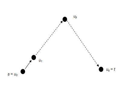
?Why is it enough to only ever climb?
Take the true shortest path from Lisbon to Berlin and look at its highest-ranked node, call it the peak. Every node between Lisbon and the peak has a lower rank than the peak, so each was contracted before it. When each of those was contracted, the shortest path through it was preserved by a shortcut between neighbours of higher rank. Repeat that argument, roughly speaking, and the whole stretch from Lisbon up to the peak collapses into a path whose ranks only go up. Likewise from Berlin to the peak. So the forward search reaches the peak with the exact distance, and so does the backward search, and adding the two gives the answer. Geisberger and co-authors proved this in the 2008 paper. The query takes, among all nodes reached by both searches, the one with the smallest total, and it can stop a search once its queue holds nothing smaller than the best total found so far.
Names on the nodes are illustrative; which junctions end up at the top depends on the preprocessing. What isn't illustrative is the result. The answer comes out as a path that's mostly shortcuts, so one last step unpacks it: each shortcut remembers the node it skipped, so it can be replaced by its two halves, and those halves unpacked in turn, until only original road edges remain. That's the turn-by-turn route Ana sees.
6.4How much it saves
This program builds a small country to try it on: an 80 × 80 grid of junctions, ordinary streets that take 50 to 70 seconds per block, and a fast road every eighth row and column that takes 20. It contracts every node in edge-difference order with lazy updates and witness searches, keeps the upward edges, and then answers 200 random routes both ways, with plain Dijkstra and with the contraction hierarchy, checking that the answers agree.
import heapq, random
random.seed(7)

# An 80 x 80 grid "country": local roads everywhere, a fast road every 8th row and column.
W = 80
def node(x, y): return y * W + x
graph = {node(x, y): {} for x in range(W) for y in range(W)}
for x in range(W):
    for y in range(W):
        for nx, ny in ((x + 1, y), (x, y + 1)):
            if nx < W and ny < W:
                fast = (y % 8 == 0 and ny == y) or (x % 8 == 0 and nx == x)
                secs = 20 if fast else random.randint(50, 70)   # seconds per block
                graph[node(x, y)][node(nx, ny)] = secs
                graph[node(nx, ny)][node(x, y)] = secs
edges = sum(len(a) for a in graph.values()) // 2

def dijkstra(s, t):
    dist, seen, pq = {s: 0}, set(), [(0, s)]
    while pq:
        d, u = heapq.heappop(pq)
        if u in seen: continue
        seen.add(u)
        if u == t: return d, len(seen)
        for v, w in graph[u].items():
            if d + w < dist.get(v, 1e18):
                dist[v] = d + w
                heapq.heappush(pq, (d + w, v))

# ---- Preprocessing: contract nodes from least to most important ----
g = {u: dict(a) for u, a in graph.items()}       # working copy that gains shortcuts
rank, up, shortcuts = {}, {}, 0

def witness(u, avoid, limit):
    """Shortest distances from u among uncontracted nodes, skipping `avoid`."""
    dist, pq = {u: 0}, [(0, u)]
    while pq:
        d, x = heapq.heappop(pq)
        if d > dist[x] or d > limit: continue
        for y, w in g[x].items():
            if y != avoid and y not in rank and d + w < dist.get(y, 1e18):
                dist[y] = d + w
                heapq.heappush(pq, (d + w, y))
    return dist

def needed(v):
    """Shortcuts we'd have to add if v disappeared."""
    nbrs = [u for u in g[v] if u not in rank]
    out = []
    for i, u in enumerate(nbrs):
        limit = max(g[v][u] + g[v][w] for w in nbrs)
        dist = witness(u, v, limit)
        for w in nbrs[i + 1:]:
            via = g[v][u] + g[v][w]
            if dist.get(w, 1e18) > via:          # no witness: v is on the only shortest path
                out.append((u, w, via))
    return out, len(nbrs)

def priority(v):
    sc, deg = needed(v)
    return len(sc) - deg                          # the edge difference

pq = [(priority(v), v) for v in graph]
heapq.heapify(pq)
while pq:
    _, v = heapq.heappop(pq)
    p = priority(v)                               # lazy update: re-check before contracting
    if pq and p > pq[0][0]:
        heapq.heappush(pq, (p, v)); continue
    for u, w, via in needed(v)[0]:
        if via < g[u].get(w, 1e18):
            g[u][w] = g[w][u] = via
            shortcuts += 1
    rank[v] = len(rank)
for u in g:                                       # keep only edges that lead upward
    up[u] = {v: w for v, w in g[u].items() if rank[v] > rank[u]}

def ch_query(s, t):
    best, settled = 1e18, 0
    dist = [{s: 0}, {t: 0}]
    pqs = [[(0, s)], [(0, t)]]
    done = [set(), set()]
    while pqs[0] or pqs[1]:
        side = 0 if (pqs[0] and (not pqs[1] or pqs[0][0] <= pqs[1][0])) else 1
        d, u = heapq.heappop(pqs[side])
        if u in done[side]: continue
        if d >= best: pqs[side] = []; continue    # nothing on this side can improve the answer
        done[side].add(u); settled += 1
        if u in dist[1 - side]:
            best = min(best, d + dist[1 - side][u])
        for v, w in up[u].items():
            if d + w < dist[side].get(v, 1e18):
                dist[side][v] = d + w
                heapq.heappush(pqs[side], (d + w, v))
    return best, settled

pairs = [(random.randrange(W * W), random.randrange(W * W)) for _ in range(200)]
dj = [dijkstra(s, t) for s, t in pairs]
ch = [ch_query(s, t) for s, t in pairs]
print(f"road graph: {len(graph):,} junctions, {edges:,} roads")
print(f"preprocessing added {shortcuts:,} shortcuts")
print(f"same answer for all 200 queries: {all(a[0] == b[0] for a, b in zip(dj, ch))}")
print(f"Dijkstra settles {sum(n for _, n in dj) / len(dj):6.0f} junctions per query (average)")
print(f"CH query settles {sum(n for _, n in ch) / len(ch):6.0f} junctions per query (average)")
s, t = node(0, 0), node(W - 1, W - 1)
print(f"corner to corner: Dijkstra {dijkstra(s, t)[1]:,}, CH {ch_query(s, t)[1]:,}")road graph: 6,400 junctions, 12,640 roads
preprocessing added 11,949 shortcuts
same answer for all 200 queries: True
Dijkstra settles 3301 junctions per query (average)
CH query settles 191 junctions per query (average)
corner to corner: Dijkstra 6,400, CH 713Check the third line first: all 200 answers are identical, so the shortcuts and the climb-only rule lost nothing. Then compare the work. Dijkstra settles about half the country per query on average, 3,301 of 6,400 junctions, and for the corner-to-corner trip it settles every single one. The contraction hierarchy settles 191 on average, about 17 times fewer, and 713 for the corner-to-corner trip. You pay for it in the second line: preprocessing roughly doubled the number of edges, from 12,640 roads to about 24,600 with the shortcuts.
A grid is a pretty poor imitation of real roads, though, because every street in a grid looks like every other and there's little hierarchy to find. Real road networks have a lot more. On the Western Europe benchmark, the 2015 survey measured a contraction hierarchy query settling about 280 nodes and taking about 0.11 milliseconds, against 9.3 million nodes and 2.2 seconds for Dijkstra: around twenty thousand times faster, for the same exact answer. Preprocessing took about five minutes, and the whole structure, graph and shortcuts together, fitted in about 0.4 GB of memory.
So Ana's route can be found in a fraction of a millisecond. But the hierarchy was built for one set of edge weights, and the jam near Heidelberg just changed one of them.
07Routing with live traffic
7.1Why traffic breaks the hierarchy
The contraction hierarchy is a snapshot of one set of travel times. Every shortcut's weight is the sum of the edges it replaced, and every witness search decided "a shortcut is needed here" or "it isn't" based on those weights. When a jam on the A5 near Heidelberg turns a ten-minute stretch into forty minutes, three things go wrong. Every shortcut that contains that stretch now has the wrong weight. Some witnesses no longer hold, so a shortcut that was skipped might now be needed. And the node order itself was chosen for the old weights, so it may no longer be a good one.
Rebuilding is the simplest fix. On the Western Europe benchmark that's about five minutes on one core, and multi-core preprocessing is faster, but traffic changes everywhere, all the time, and a hierarchy for the whole world takes much longer: chapter 50 quoted Uber in 2015 estimating about 12 hours to build one for all the world's roads. By the time the rebuild finishes, the jam it was meant to include has moved. OSRM's documentation says the same about its own pipeline: feeding new traffic speeds to a contraction hierarchy means re-running the contraction, which it calls "too slow for big datasets".
What we want is a structure whose expensive part depends only on the shape of the road network, which changes slowly, while the part that depends on travel times can be recomputed in seconds.
7.2Customizable route planning
That's the idea behind customizable route planning (CRP), published by Daniel Delling, Andrew Goldberg, Thomas Pajor and Renato Werneck at Microsoft Research in 2011. It splits the work into three phases.
The first phase, partitioning, cuts the road network into cells, compact regions of the map, choosing the boundaries so that as few roads as possible cross between cells. Road networks are good at this, because natural barriers do the work: rivers with few bridges, mountains with few passes, borders with few crossings. The nodes where roads cross a cell boundary are its boundary nodes. Then it does the same again at a coarser level, grouping cells into bigger cells, for several levels. This phase uses only the shape of the network, not travel times, so it runs rarely, when roads are added or removed, and can take as long as it needs; on Western Europe the 2015 survey reports about an hour.
The second phase, customization, takes the current travel times and, for every cell, computes the fastest way through it between every pair of its boundary nodes. Those become shortcut edges, a small complete table per cell, and together the boundary nodes and their shortcut tables form an overlay graph on top of the cells. Cells are processed bottom-up, the smallest first, and each one independently, so they can all run in parallel. On Western Europe this took about 0.37 seconds on a 12-core server.
Last comes the query. A bidirectional search explores normally inside the cells containing Ana's café and the Brandenburg Gate, and everywhere else moves only on the overlay graph, jumping across whole cells, and at the coarse levels whole regions, in one step. On Western Europe a query settled about 2,800 nodes and took about 1.7 milliseconds. That's slower than a contraction hierarchy's 0.11 ms, but still fast enough to answer any route, and it was nearly as fast with turn costs and with other cost functions, where contraction hierarchies slow down.
The Scene simplifies one thing: real systems usually recompute all cells on a fixed schedule, since that's fast enough, instead of tracking which are dirty. Either way, the slow, shape-dependent part is done once, and the fast, weight-dependent part is redone as often as traffic changes.
Which routing structure should serve routes with live traffic?
- Fastest queries: about 0.11 ms on Western Europe
- Minutes of preprocessing for a continent
- Any weight change means re-contracting
- Slower with turn costs and unusual cost functions
- New travel times applied in under a second for a continent
- Robust to turn costs and different cost functions
- Queries about ten times slower than CH (still milliseconds)
- A partition step that must be rerun when roads change
- Always uses the latest weights
- Simple
- Explores millions of nodes across a continent
- Too slow per query at scale
Microsoft deployed CRP in Bing Maps, announced in 2012, and OSRM added its own version, called multi-level Dijkstra (MLD), whose documentation now recommends it in general and singles it out for regular traffic updates: partition once, then rerun only osrm-customize with new speeds. A later variant, customizable contraction hierarchies (2014), gets the same split by fixing a weight-independent contraction order. Google hasn't published which routing algorithm it runs in production. A design for Ana's question needs this property, whatever its name: a precomputation that depends only on the shape of the network, and a fast step that applies new travel times.
There's one more thing the route needs that we've glossed over. Customization folds in "the current travel times". The next question is where those come from.
08Where traffic comes from
8.1Every phone is a speed sensor
Traffic used to be measured with equipment in the road: induction loops cut into the tarmac, cameras and radar at fixed points. They're accurate, but they're expensive, so they cover motorways and a few major roads, and say nothing about the side street where a delivery van has stopped.
Google's answer, announced in August 2009, was to use the phones already in the cars. When users turn on Google Maps with location enabled, the post explained, "your phone sends anonymous bits of data back to Google describing how fast you're moving", and combining "the speed of other phones on the road, across thousands of phones moving around a city at any given time" gives "a pretty good picture of live traffic conditions". A phone reporting its position and speed this way is called a probe.
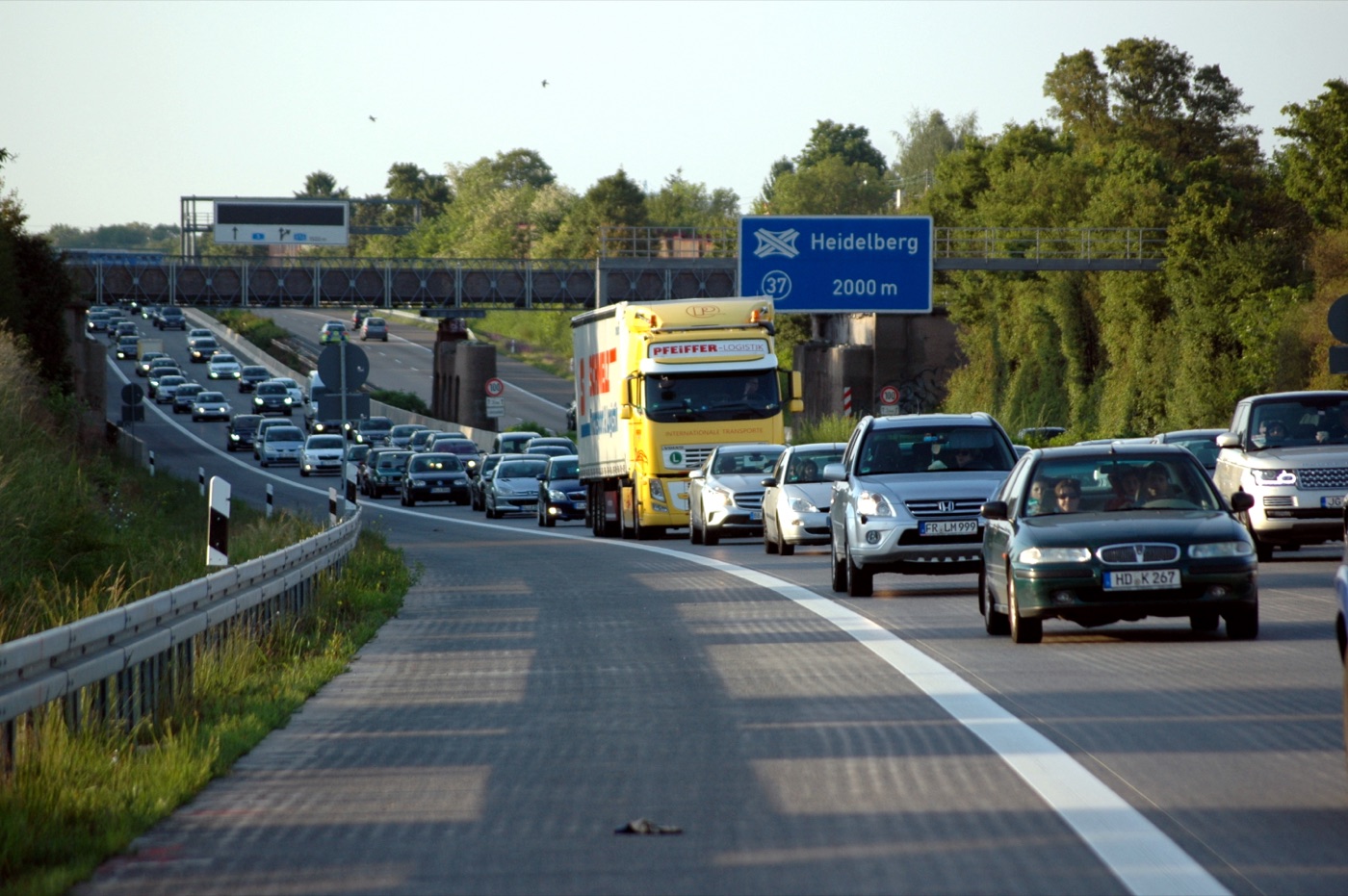
Raw positions aren't speeds on roads yet. A GPS fix is good to a few metres in the open and much worse between tall buildings, and a motorway often runs right beside a slow service road or under a bridge carrying another road. So the first processing step, map matching, works out which road segment each probe is on, and in which direction, by fitting the whole sequence of a phone's positions to a path a car could drive, instead of snapping each point to the nearest line on its own. Only then can the probe's speed be credited to the right segment.
Next, speeds are combined. For each segment, in each direction, the probes that crossed it in the last couple of minutes are averaged into one current speed, with outliers dropped (a postal van stopping at every door isn't traffic). A segment with too few probes has no live estimate, and falls back on its history: what its speed usually is at this hour on this day of the week.
?Isn't that a record of where everyone drives?
It would be, and Google's 2009 post addressed it directly. It described three protections: speed and location are collected only from users who've enabled location, data from many phones in the same area is combined "to make it hard to tell one phone from another", and "we find the start and end points of every trip and permanently delete that data so that even Google ceases to have access to it". The start and end of a trip are the points that identify someone, their home and their workplace; the middle of a motorway is shared by thousands. Aggregation by segment helps twice: it makes the data more private and more accurate at the same time.
8.2Live speeds and historical patterns
Live speeds say what the road is like now. Ana's route also needs what roads will be like when she gets to them, and for that the system keeps historical traffic patterns: for each segment, its typical speed for each time of day and day of week, learned from months of past probes. Google's 2020 description gives an example: a Northern California freeway that typically runs at 65 mph between 6 and 7 am may be down to 15–20 mph in the late afternoon.
History has to be kept current, too. When lockdowns began in early 2020, Google saw "up to a 50 percent decrease in worldwide traffic", and patterns learned from 2019 suddenly predicted jams that no longer happened. Google said it responded by giving more weight to the last two to four weeks of patterns and less to older ones.
Google's 2020 post lists the other inputs beside probes: road quality and size, speed limits, tolls and restrictions from local governments, and reports from users about closures, construction and broken-down vehicles.
Where should traffic data come from?
- Accurate, continuous counts at each sensor
- No personal data involved
- Expensive, so mostly on motorways
- Blind to the streets between sensors
- Covers every road where people drive with the app
- Coverage grows with users at no extra cost
- Sparse on quiet roads and at night
- Needs privacy protections and map matching
- Each source covers another's gaps
- Incidents show up before speeds drop
- Several pipelines to run and reconcile
Google's 2009 and 2020 posts describe exactly this mix: aggregate location data from phones as the backbone, authoritative data from local governments for speed limits and closures, and user reports of incidents. The more people use the app, the better the traffic data gets, which is part of why a map with two billion users is hard to compete with.
09Predicting the arrival time
9.1Adding up today's speeds isn't enough
With the route found, the app has to say when Ana will arrive. Here's the obvious design: walk along the route's segments, look up each one's current travel time, and add them up.
That's wrong in a way that matters most on exactly the trips where people check the ETA. The jam near Heidelberg is a problem now, but Ana won't get there for many hours, by which time it will probably be gone. Meanwhile the bridge into Berlin is clear now, but she'll reach it in the evening rush. Adding up current travel times assumes conditions now will last the whole trip.
The fix is to walk the route forward in time: look up each stretch at the moment the car will reach it, which depends on how long all the stretches before it took. This program compares the two on a shorter route with a jam that's clearing and a bridge where the rush is building:
# One route as a list of stretches of road. For each, a function giving how many
# minutes it takes to drive if you enter it t minutes from now.
def steady(minutes):
    return lambda t: minutes

def jam_clearing(now, normal, clears_at):
    # slow now, easing back to normal by `clears_at` minutes from now
    return lambda t: normal if t >= clears_at else now - (now - normal) * t / clears_at

def rush_hour_builds(normal, peak, starts, peak_at):
    # clear now; the evening rush builds from `starts` to `peak_at` minutes from now
    def f(t):
        if t <= starts: return normal
        if t >= peak_at: return peak
        return normal + (peak - normal) * (t - starts) / (peak_at - starts)
    return f

route = [
    ("city streets",     steady(9)),
    ("ring road",        steady(7)),
    ("motorway, jammed", jam_clearing(now=30, normal=8, clears_at=20)),
    ("motorway",         steady(31)),
    ("bridge into town", rush_hour_builds(normal=5, peak=20, starts=45, peak_at=75)),
    ("last streets",     steady(6)),
]

print(f"{'stretch':18} {'now':>5} {'enter at':>9} {'takes':>6}")
t = 0.0
for name, f in route:
    m = f(t)                       # look the stretch up at the time you'll reach it
    print(f"{name:18} {f(0):5.1f} {t:9.1f} {m:6.1f}")
    t += m

print(f"ETA from current speeds:     {sum(f(0) for _, f in route):.0f} min")
print(f"ETA walking forward in time: {t:.0f} min")stretch now enter at takes
city streets 9.0 0.0 9.0
ring road 7.0 9.0 7.0
motorway, jammed 30.0 16.0 12.4
motorway 31.0 28.4 31.0
bridge into town 5.0 59.4 12.2
last streets 6.0 71.6 6.0
ETA from current speeds: 88 min
ETA walking forward in time: 78 minThe "now" column is what each stretch takes at this moment; "enter at" is when the car gets there. The jammed motorway takes 30 minutes now, but the car reaches it at minute 16, when the jam has mostly cleared, so it takes roughly 12. Meanwhile the bridge takes 5 minutes now, but the car reaches it at minute 59, in the rush, and it takes about 12. The current-speed ETA is wrong twice, in opposite directions, and ends up ten minutes out overall. Errors that happen to cancel would be no comfort either, because they wouldn't cancel on the next route.
The forward walk is only as good as the functions it calls, though, and in the program they're made up. Nobody can know in advance how fast the jam will clear. Predicting each stretch's travel time at a future moment is the hard part, and it's a prediction problem: given what the road looks like now and what it usually looks like, guess what it will look like in twenty minutes.
9.2A graph neural network for travel times
In September 2020 DeepMind and Google described the model that does this in Google Maps, and the full paper, ETA Prediction with Graph Neural Networks in Google Maps by Austin Derrow-Pinion and co-authors, appeared at the CIKM conference in 2021.
Its first idea is about what to predict for. Predicting each tiny road segment separately misses how traffic moves: a jam on one segment spills backward onto the segments behind it, and a slow exit ramp slows the lane leading to it. So the model works on supersegments, sequences of connected road segments that follow typical routes and share a lot of traffic. In 2021 the paper reported about a million predefined supersegments, covering most freeways, major arterial roads and popular short-cuts in cities. Less busy streets aren't covered, and use simpler per-segment models.
Its second idea is the model itself. A supersegment is a small graph: each road segment is a node, and edges connect segments that follow one another or meet at a junction. A graph neural network (GNN) is a model that works on such a graph by message passing: each node starts with a vector of numbers describing its segment, then repeatedly sends messages to its neighbours and updates its own vector from the messages it receives. After a few rounds, each segment's vector reflects what's happening on the segments around it, which is how a jam ahead of a segment can affect the prediction for it. Finally, the model predicts the supersegment's travel time.
The inputs are the two kinds of data from section 8. For each segment, the paper lists its length and road class; its real-time speeds and travel times for each of the 17 two-minute windows before the prediction, about half an hour of recent history; and its historical speeds for five eight-minute windows before and seven after, averaged over the past 17 weeks. It predicts travel times for several fixed horizons, how far into the future the car will enter the supersegment, which is exactly what section 9.1's forward walk needs.
The results were large for a system already accurate on over 97% of trips. DeepMind's 2020 post reported accuracy improvements of up to 50% in cities including Berlin, Jakarta, São Paulo, Sydney, Tokyo and Washington DC, and the paper reported reducing "negative ETA outcomes", predictions off by more than a threshold, by over 40% in cities like Sydney, compared to the previous production system. Training was unstable at first, because batches mixed graphs of very different sizes, and the team stabilised it with MetaGradients, a technique in which the model learns its own learning rate during training.
?How can a neural network answer within a route request's time limit?
It doesn't run during the request. The paper describes the engineering: running the network on every supersegment of every route on the fly was "not practical nor scalable", so a background job runs it for every predefined supersegment at a fixed set of horizons and stores the predictions in a shared lookup table, refreshed periodically. When Ana's route request arrives, the server walks her route forward in time as in section 9.1, fetching each supersegment's predictions from the table and interpolating between the two horizons either side of when she'll get there. Google tested refreshing the table every 15 seconds and saw no measurable loss of accuracy with refreshes as slow as every two minutes, so staleness wasn't a problem.
That is the same move the tile servers made in section 2 and the routing graph in section 6: take the expensive computation out of the request, run it in the background for a fixed set of keys (tiles, shortcuts, supersegment-horizon pairs), and make the request a lookup.
How should the ETA be computed?
- Trivial and fast
- Always uses the latest data
- Wrong whenever conditions change during the trip
- No notion of a jam spreading or clearing
- Captures rush hours
- Cheap lookups
- Blind to today's accident or closure
- Goes stale when habits shift, as in 2020
- Combines today's conditions with usual patterns
- Captures jams spreading between connected segments
- A table lookup at request time
- A training and serving pipeline to run
- Coverage only on the predefined supersegments; fallbacks elsewhere
Google's production ETA used this design from 2020. For Ana's day-long drive, the horizons for most of the route are hours away, where live data has little to say, so the prediction relies almost entirely on historical patterns for those stretches; the model matters most for the first hour, where today's conditions are still informative. Chapter 50's Uber made the same choice of learning a correction on top of a road-graph estimate, from the opposite side: DeepETA predicts the error of the whole route's sum, where Google's model predicts each supersegment's time.
10The whole system
10.1Every box, and why it's there
| Component | What it does | Added because |
|---|---|---|
| Tile pyramid | A fixed z/x/y grid of the world at every zoom | Per-screen images can't be cached (§2.1) |
| Tile CDN and on-demand rendering | Draw each tile once, serve it from caches near users | Popularity is very uneven; most tiles are never viewed (§2.4) |
| Vector tiles | Send geometry; the phone draws | Smooth zoom and rotation, much less data (§3) |
| Search | Prefix index plus ranking; reverse geocoding | Text must become a point before routing (§4) |
| Overlay graph (CRP) | Precomputed shortcuts per cell, recomputed with traffic | Dijkstra is seconds per route; CH can't take live weights (§5–7) |
| Traffic pipeline | Probes → map matching → per-segment speeds | Sensors don't cover most roads (§8) |
| ETA lookup | GNN predictions per supersegment and horizon, refreshed in the background | Current speeds mispredict trips that last longer than a jam (§9) |
10.2From top to bottom
| Level | The choice | Data structure or algorithm |
|---|---|---|
| System | Move expensive work off the request path | Precomputed tiles, shortcuts and predictions; requests are lookups |
| Map projection | Web Mercator, cut at ±85.0511° | Square world; x linear in longitude, y = asinh(tan φ) |
| Tile addressing | A quadtree of 256-pixel squares | z/x/y: 4z tiles per level, parent = half of x and y |
| Tile encoding | Geometry, not pixels | Protocol Buffers; command integers (id & 7) | (count << 3); zigzag deltas on a 4096 grid |
| Search | Suggest while typing | Trie with stored top completions; importance ranking |
| Routing, static | Exploit road hierarchy | Contraction hierarchy: node order by edge difference, witness searches, climb-only bidirectional Dijkstra |
| Routing, live | Separate shape from weights | Multilevel partition, per-cell boundary-to-boundary shortcut tables, parallel customization |
| Traffic | Aggregate probes per segment | Map matching; per-segment, per-direction windows; historical profiles |
| ETA | Predict per supersegment, ahead in time | Graph neural network, message passing, multiple horizons, lookup table |
11What goes wrong, and what it cost
11.1Failures this design has to survive
| What happens | What the user sees | What the design does |
|---|---|---|
| A road is edited | The old map for a while | Affected tiles re-render at the origin; cached copies expire on their own schedule |
| A rarely viewed tile is requested | A short wait for that square | Rendered on demand as part of a metatile, then cached |
| The CDN loses a region | Slower tiles nearby | Requests go to other edge servers or the origin; tiles are immutable, so any copy will do |
| A sudden jam | Red on the map; maybe a new route | Probes update segment speeds within minutes; customization updates the overlay graph |
| Too few probes on a road | Traffic shown as normal | Historical patterns fill in; quiet roads are where errors are cheapest |
| Habits change suddenly (2020) | ETAs that expect jams that never come | Weight the last few weeks more heavily in historical patterns |
| GPS jumps between parallel roads | A phantom jam on the wrong road | Map matching fits the whole trace, not single points; outliers are dropped |
11.2The tradeoffs, in one table
| Decision | Chosen | Given up | Why it was worth it |
|---|---|---|---|
| What the client asks for | Fixed tiles by z/x/y | Pixel-perfect screens from the server | Identical requests can be cached by everyone |
| When tiles are drawn | On demand, in metatiles, then cached | Instant first view of rare tiles | Work is spent only where people look |
| Raster or vector | Vector (Google, 2010) | Simple clients | Smooth zoom and rotation; over 100× less data across zooms |
| Static routing | Contraction hierarchies | Minutes of preprocessing; double the edges | About 20,000× fewer settled nodes than Dijkstra |
| Live routing | Customizable route planning | About 10× slower queries than CH | New traffic weights applied in under a second |
| Traffic source | Phones as probes, plus official data and reports | Simple, privacy-free sensors | Coverage of every road people drive |
| ETA | Cached GNN predictions over supersegments | A simple sum | Up to 50% better accuracy in some cities (2020) |
12Summary
- Per-screen map images can't be cached, because no two screens are the same; a fixed grid of tiles makes everyone ask for the same pieces.
- Web Mercator makes the world a square by cutting it at ±85.0511°, keeping north up and angles true at the cost of inflating areas near the poles.
- A tile is named by z/x/y: 4z tiles at zoom z, and two short formulas turn a latitude and longitude into one.
- Tiles are rendered on demand and cached everywhere, because a small set of tiles is wildly popular and most are never seen; OpenStreetMap's CDN served about 97% of tile bytes from cache in 2025.
- Vector tiles send geometry instead of pixels, as delta- and zigzag-encoded drawing commands, so the phone can zoom, rotate and restyle smoothly with far less data.
- Dijkstra explores everything closer than the destination, about 9.3 million nodes and two seconds for a random trip across Western Europe, and A* with a straight-line guess barely helps on travel times.
- Contraction hierarchies add shortcuts around unimportant nodes in edge-difference order, so a query only climbs from each end and meets at the top, settling a few hundred nodes.
- Live traffic breaks a hierarchy's precomputed weights; customizable route planning separates the network's shape (slow, rare) from its weights (fast, frequent), and applies new traffic to a continent in under a second.
- Traffic comes from phones as probes, map-matched to segments and aggregated per direction over short windows, with trip ends deleted and history filling the gaps.
- An ETA must walk forward in time, asking each stretch how slow it will be when the car arrives, not how slow it is now.
- Google predicts those times with a graph neural network over supersegments, precomputed for fixed horizons into a lookup table, so the request stays a lookup.
13Build this
A tiny map service of your own.
- Download a small OpenStreetMap extract of a city from Geofabrik, run OSRM on it twice, once with the CH pipeline (
osrm-extract,osrm-contract) and once with MLD (osrm-extract,osrm-partition,osrm-customize), and compare preprocessing time and query latency for a few hundred random routes. - Make a CSV of segment speeds that slows one major road to a crawl. Apply it to both pipelines with
--segment-speed-fileand time how long each takes to absorb the change. Check that routes now avoid the road. - Extend the contraction hierarchy program in section 6.4 to record, for every shortcut, the node it skipped, and unpack the corner-to-corner route into original edges. Check its length against Dijkstra's path.
- Write the tile function from section 2.3 in reverse (tile to latitude and longitude of its corners), and draw the outlines of every zoom-12 tile your city touches.
- Change section 9.1's route so the current-speed ETA happens to be right, then change the departure time by twenty minutes and watch it go wrong again.
14Interview questions
beginnerWhy do web maps use tiles at all, instead of rendering exactly what's on the screen?›
Because no two screens show exactly the same box of the world, so images rendered per screen can't be shared or cached, and every drag would need a fresh database query and render. A fixed grid of tiles at fixed zoom levels, named by z/x/y, means everyone looking at the same area asks for the same files. Each tile can be rendered once and served from caches and a CDN to everyone, which turns a rendering problem into a caching problem.
beginnerWhy Web Mercator, given how badly it distorts Greenland?›
Web Mercator keeps north straight up and preserves angles locally, so streets meet at the right angles and a local area looks undistorted at any zoom, and that's what you need to find your way. Its distortion is in area, which grows towards the poles; that matters for a world atlas and hardly at all for street navigation. Cutting it at about 85.05° makes the flattened world exactly square, which makes the tile grid simple.
intermediateHow would you convert a latitude and longitude to a tile, and find its parent and children?›
At zoom z there are 2^z tiles across. x is the longitude's position from 180° west as a fraction of 360°, times 2^z, rounded down. y uses the Mercator formula: (1 − asinh(tan φ)/π)/2 × 2^z, rounded down, counting from the top. The parent at zoom z − 1 is (x/2, y/2) rounded down, and the four children at zoom z + 1 are (2x, 2y), (2x + 1, 2y), (2x, 2y + 1) and (2x + 1, 2y + 1). It's a quadtree addressed by arithmetic.
intermediateRaster or vector tiles: what are the tradeoffs?›
Raster tiles are finished images: any client can show them and the result is identical everywhere, but they only look right at whole zoom levels, labels can't rotate with the map, and every style is a separate set. Vector tiles carry geometry and tags, encoded compactly (delta- and zigzag-encoded commands in Protocol Buffers), and the client draws them, which allows smooth zoom, rotation, 3D and restyling with far less data; the cost is a capable client and a rendering engine on every platform. Google moved its Android app to vector tiles in 2010; OpenStreetMap's standard layer is still raster.
intermediateExplain contraction hierarchies.›
Preprocessing ranks nodes by importance and contracts them from least important to most: removing a node and adding a shortcut between each pair of its neighbours whose only shortest path went through it, which a small witness search checks. The order is chosen greedily by edge difference (shortcuts added minus edges removed), updated lazily, so dead ends go first and motorway junctions last. A query runs bidirectional Dijkstra that only follows edges to higher-ranked nodes; the highest node on the shortest path is reached exactly by both searches, so the minimum of forward plus backward distance is the answer. On Western Europe that's a few hundred settled nodes and about a tenth of a millisecond, versus millions and seconds for Dijkstra.
deepHow do you keep routing fast when travel times change every few minutes?›
Separate what depends on the network's shape from what depends on its weights. Customizable route planning partitions the graph into cells with few boundary nodes, once, which is slow but rarely needed. Customization then recomputes, for every cell, the shortest distances between its boundary nodes under the current weights, bottom-up through several levels and in parallel; on Western Europe that took about 0.37 seconds on 12 cores in published experiments. Queries search normally near the endpoints and on the overlay of cell shortcuts elsewhere, in a millisecond or two. Contraction hierarchies are faster per query but would need re-contracting for every weight change. OSRM's MLD and Bing Maps use this design.
deepHow would you predict the ETA for a long drive?›
Walk the route forward in time: for each stretch, predict its travel time at the moment the car will reach it, which depends on all earlier stretches. Near the start, live speeds from phones are informative; hours ahead, historical patterns for that hour and weekday dominate. Google's production model is a graph neural network over supersegments of connected road segments, fed with recent two-minute speed windows and 17-week historical averages, predicting several horizons ahead. Because running it per request would be too slow, predictions for every supersegment and horizon are precomputed into a lookup table refreshed every few seconds to minutes, and the request interpolates between horizons.
15Go deeper
At zoom 10, Lisbon is in tile (486, 392). What's its parent tile at zoom 9, and how many zoom-12 tiles lie inside it?›
The parent is (243, 196), each number halved and rounded down. Each zoom level splits a tile into four, so two levels down there are 4 × 4 = 16 zoom-12 tiles inside it.
In a contraction hierarchy, why can't the two searches stop as soon as they first meet?›
The first node reached by both searches isn't necessarily the highest-ranked node on the shortest path, so its total may not be the best. The searches continue until neither queue holds a distance smaller than the best total found so far.
A jam appears on one motorway segment. With customizable route planning, what has to be recomputed?›
Only the shortcut tables of the cell containing that segment, and of the larger cells that contain that cell at coarser levels. The partition, and every other cell's tables, stay as they were.
The survey behind most numbers in sections 5 to 7: Dijkstra, A*, ALT, contraction hierarchies, CRP and hub labels, compared on the same Western Europe graph.
The original paper: node ordering, witness searches, and the proof that the climb-only query is exact.
Separating metric-independent preprocessing from customization, so live traffic can be applied to a continent in under a second.
Supersegments, features, MetaGradients, and the cached lookup table that makes the model servable. The DeepMind blog post (September 2020) is the short version.
Why Google moved from 256-pixel image tiles to vector tiles, with the 360 billion tiles and 100× less data figures.
The tile formulas, zoom tables and code in many languages; and the open vector tile encoding, command by command.
Both routing pipelines, CH and MLD, side by side, and how to feed them live speeds.
16Related chapters
Geohash, quadtrees, S2 and H3, the road graph, and Uber's own routing engine and DeepETA. Chapter 50.
Expiry, invalidation and hit rates, the machinery behind serving tiles. Chapter 25.
How CDN edge servers are found and what they do. Chapter 35.
The streams that carry probe data into per-segment speeds. Chapter 23.
Cutting data into pieces with few cross-links, the same goal as CRP's graph partition. Chapter 29.