You're on an outdoor-gear shop's website, and you type running shoes into the search box at the top. Before you've lifted your finger from the Enter key, a page of results appears: ten pairs of shoes, the most relevant first, and a line saying there are thousands more. The shop sells about ten million products, from tent pegs to snowshoes, and it found the right ten in a few tens of milliseconds.
If you have built a website backed by a database, your first idea for that search box was probably a query like WHERE title LIKE '%running shoes%'. That query is slow on ten million rows, and it is also wrong in ways that have nothing to do with speed. It can't find "Lightweight road running shoe", because the title says shoe and you typed shoes. It happily returns snowshoes when you ask for shoes. And when it does find matches, it returns them in whatever order the rows happen to be stored, with no idea which one you'd most like to see.
A search engine is the program built to do this job properly. Elasticsearch, OpenSearch and Solr are the ones you're most likely to meet, and all three are built on a library called Lucene. This chapter follows your query through one, asking a single question the whole way: how does typing a few words return the ten best products out of ten million in milliseconds? The short answer is that almost all the work happens before you type, when the engine builds an index that maps every word to the products that contain it. The rest of the chapter builds that index step by step, then shows how the engine ranks what it finds, keeps the index up to date, and spreads it across machines.
01Why the database can't just look
1.1Six products and a LIKE query
Let's start with a catalogue small enough to hold in your head. Our shop has six products, and the database stores them in a table with an id and a title:
| id | title |
|---|---|
| 1 | Men's trail running shoes |
| 2 | Waterproof running jacket |
| 3 | Lightweight road running shoe |
| 4 | Hiking boots, waterproof leather |
| 5 | Running socks, 3 pairs |
| 6 | Aluminium snowshoes |
Somebody searching for running shoes wants products 1 and 3, and might be glad to see the socks. They don't want the snowshoes. Let's see what the obvious SQL does with this, using SQLite, the small database that ships inside Python. LIKE compares a column against a pattern, and % in the pattern stands for "any run of characters", so '%shoe%' matches any title with shoe somewhere inside it. It also creates an ordinary index on title, then asks SQLite how it plans to run the query with EXPLAIN QUERY PLAN. Last, it adds a million filler rows and times the same kind of query.
import sqlite3, time

db = sqlite3.connect(":memory:")
db.execute("create table products(id integer primary key, title text)")
db.execute("create index by_title on products(title)")
db.executemany("insert into products(title) values (?)", [
    ("Men's trail running shoes",),
    ("Waterproof running jacket",),
    ("Lightweight road running shoe",),
    ("Hiking boots, waterproof leather",),
    ("Running socks, 3 pairs",),
    ("Aluminium snowshoes",),
])
q = "select id, title from products where title like ?"
print("'%running shoes%' ->", db.execute(q, ("%running shoes%",)).fetchall())
print("'%shoes running%' ->", db.execute(q, ("%shoes running%",)).fetchall())
print("'%shoe%'          ->", db.execute(q, ("%shoe%",)).fetchall())
print("plan:", db.execute("explain query plan " + q, ("%shoe%",)).fetchall()[0][3])

# the same query over a million rows
db.executemany("insert into products(title) values (?)",
               ((f"product {i} in colour {i % 97}",) for i in range(1_000_000)))
t = time.perf_counter()
n = len(db.execute(q, ("%running shoe%",)).fetchall())
print(f"1,000,006 rows: {n} matches in {(time.perf_counter() - t) * 1000:.0f} ms")'%running shoes%' -> [(1, "Men's trail running shoes")]
'%shoes running%' -> []
'%shoe%' -> [(1, "Men's trail running shoes"), (3, 'Lightweight road running shoe'), (6, 'Aluminium snowshoes')]
plan: SCAN products
1,000,006 rows: 2 matches in 41 msRead the output line by line. The pattern '%running shoes%' finds only product 1, because product 3 says shoe and the pattern needs the exact characters running shoes in a row. Swap the words and nothing matches at all. Loosen the pattern to '%shoe%' and you get product 3 back, along with the aluminium snowshoes, because LIKE matches characters and has no idea where one word ends and another begins. None of the results come with any sense of which is better.
Now look at speed. SCAN products means SQLite reads every row and tests each title against the pattern. On a million rows that took about 40 milliseconds. Timings vary by machine, but the time grows with the size of the table, so the shop's ten million products would take ten times as long, for every search.
1.2Why an ordinary index doesn't help
SQLite ignored the index on title. Chapter 18 explains what that index is: a B+tree, a tree of pages that keeps the titles sorted so the database can find one by walking down from the root, the way you find a word in a dictionary by its first letters. Sorting by the whole title only helps when you know how the title starts. A pattern that begins with % says "anything can come first", so the sorted order is useless, and the database falls back to reading everything.
?Couldn't we make LIKE smarter?
We could lowercase everything, strip plurals, and search for each word with its own LIKE, but each fix is another pass over every row. The underlying problem is the direction of the lookup. A table is organised by product: given a product, it tells you the words in its title. A search needs the opposite: given a word, which products contain it? We need a different data structure, built ahead of time, organised by word.
Before we can build that, we have to decide what counts as a word. Is Shoes the same word as shoes? Is shoe the same as shoes? What about Men's?
02From text to terms
2.1Tokens
The first step is to cut each title into pieces. Most engines start with the obvious rule: split wherever there's a space or punctuation, and turn every letter into lowercase so that Running and running come out the same. Each piece is called a token. Product 1, "Men's trail running shoes", becomes five tokens: men, s, trail, running, shoes. Splitting at the apostrophe left a stray s, which will need dealing with.
Real tokenizers are more careful. Lucene's standard tokenizer follows the Unicode standard's rules for where words begin and end, so it knows that 3.5mm is one token. For an English catalogue, though, splitting and lowercasing gets you most of the way.
2.2Stop words
Some tokens carry almost no meaning on their own. Words like the, of, for and and appear in nearly every piece of English, so knowing that a product title contains for tells you nothing about whether it's the product you want. These are called stop words, and an engine can be told to throw them away.
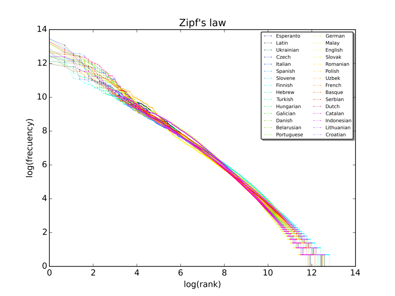
The few most common words make up a large fraction of all the tokens in any collection, so dropping them makes the index noticeably smaller, which mattered when disks were small. It has a cost: "to be or not to be" is made entirely of stop words. Today's engines usually keep them and let the ranking function from section 6 give them very little weight; the standard analyzer in Elasticsearch and OpenSearch keeps them by default. For our tiny catalogue we'll drop a short list, with that stray s added.
2.3Stemming
Still, shoes doesn't match shoe. To fix that, we cut each token back to a shared root, so that shoes, shoe and perhaps shoeing all become the same thing. This is called stemming, and the program that does it is a stemmer.
A minimal stemmer only removes plural endings. Lucene's EnglishMinimalStemmer implements Donna Harman's 1991 "S-stemmer" in a dozen lines: drop a final s, turn ies into y, and leave words alone when the ending looks like part of the word. An aggressive stemmer, the best known being Martin Porter's algorithm from 1980, strips many suffixes in several rounds, so running becomes run. Elasticsearch's and OpenSearch's English analyzer uses Porter's.
Let's run both. Our S-stemmer follows Lucene's code line for line. For Porter we borrow SQLite's: its full-text search module, FTS5, can stem with Porter's algorithm, and a companion table, fts5vocab, reads back the terms it stored.
import re, sqlite3

def s_stem(w):
    # Harman's S-stemmer, the rules in Lucene's EnglishMinimalStemmer
    if len(w) < 3 or w[-1] != "s" or w[-2] in "us":
        return w
    if w.endswith("ies") and len(w) > 3 and w[-4] not in "ae":
        return w[:-3] + "y"
    if w[-2] == "e" and w[-3] in "iaoe":
        return w
    return w[:-1]

# SQLite's FTS5 ships Porter's stemmer; we read back the terms it stores
db = sqlite3.connect(":memory:")
db.execute("create virtual table p using fts5(t, tokenize='porter unicode61')")
db.execute("create virtual table v using fts5vocab(p, 'instance')")
def porter(text):
    doc = db.execute("insert into p(t) values (?)", (text,)).lastrowid
    return [t for (t,) in db.execute(
        "select term from v where doc = ? order by offset", (doc,))]

for text in ["Men's trail running shoes", "Running socks, 3 pairs",
             "batteries glasses", "Aluminium snowshoes",
             "university universe", "generous generation"]:
    tokens = re.findall(r"[a-z0-9]+", text.lower())
print(f"{text:26} S: {' '.join(s_stem(t) for t in tokens):24} Porter: {' '.join(porter(text))}")Men's trail running shoes S: men s trail running shoes Porter: men s trail run shoe
Running socks, 3 pairs S: running sock 3 pair Porter: run sock 3 pair
batteries glasses S: battery glasse Porter: batteri glass
Aluminium snowshoes S: aluminium snowshoes Porter: aluminium snowsho
university universe S: university universe Porter: univers univers
generous generation S: generous generation Porter: gener generThe first line holds a surprise: the minimal stemmer leaves shoes alone. Harman's rules treat a word ending in -oes as possibly a word in its own right (does, toes), so our running example wouldn't match. Porter turns shoes into shoe and running into run. Stems like glasse and batteri look odd, but nobody ever sees a stem. The only requirement is that the same word always produces the same stem, at indexing time and at search time.
Aggressive stemming has a price, too. Porter maps university and universe to univers, so a search for one finds the other. That's overstemming, and the opposite failure, leaving related words apart (the S-stemmer with shoes), is understemming. Every stemmer trades one against the other, which is why engines let you pick per field.
2.4The analyzer
Splitting, lowercasing, removing stop words and stemming run one after another, as a pipeline. The whole pipeline is called an analyzer, and what comes out the end are terms: the units the index is built from. From now on, our analyzer is Porter's stemmer with a short stop list, so product 1 becomes the terms men trail run shoe, and the query running shoes becomes run shoe.
Each product is now a short list of terms, still organised by product. Next, we turn it around.
03The inverted index
3.1Turning the table around
Think about the index at the back of a textbook. You look up photosynthesis and it gives you page numbers: 41, 87, 203. A book is organised by page, and the index is the same information organised by word. A search engine builds exactly that: for every term, a list of the documents that contain it.
That structure is called an inverted index, because it inverts the document-to-words direction of the table. It has two parts. The term dictionary is the sorted list of every distinct term. Each term points to its postings list, the list of documents that contain it, and each entry in that list is a posting.
Documents are identified in postings by a doc ID, a small whole number the engine assigns as documents arrive: 0, 1, 2 and so on, with no gaps. (Lucene numbers from 0; we'll number our products 1 to 6 to match the table.) Small dense numbers keep every posting compact, and assigning them in arrival order means each postings list stays sorted by doc ID just by appending to it. That sorting pays off in sections 4 and 5.
To answer running shoes, the engine looks up two terms and reads two short lists. It never looks at product 4 or product 6. However many products the shop sells, the work depends on the length of those two lists.
3.2What else a posting holds
A posting that says "doc 3 contains shoe" tells us whether a product matches. Two more things belong alongside it. The first is how many times the term appears in that document, its term frequency, which section 6 uses for ranking. The second is where the term appears, as a position: the first term is at position 0, the second at 1, and so on. Positions let the engine answer a phrase query like "trail running", which section 10 does.
The dictionary also stores, for each term, how many documents contain it, the length of its postings list. That's the term's document frequency, written df: run has a df of 4 in our catalogue, jacket a df of 1.
3.3Building one
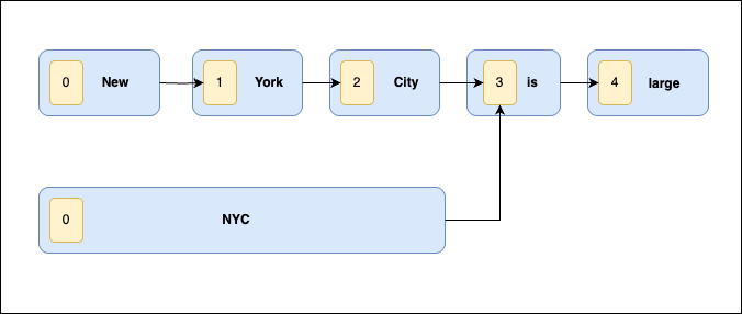
Building an inverted index is a single pass over the documents. Take each document in doc ID order, run its text through the analyzer, and for every term it produces, append the doc ID and position to that term's postings. Here is the moment product 3 goes in:
Every append went on the end of a list, because doc IDs are handed out in increasing order. Section 8 comes back to what happens when products change after the index is built. Here is the whole thing in code, with SQLite's Porter stemmer as the analyzer; it prints every term with its df and postings, written doc:[positions].
import sqlite3
from collections import defaultdict

products = {
    1: "Men's trail running shoes",
    2: "Waterproof running jacket",
    3: "Lightweight road running shoe",
    4: "Hiking boots, waterproof leather",
    5: "Running socks, 3 pairs",
    6: "Aluminium snowshoes",
}
STOP = {"a", "an", "and", "for", "in", "of", "on", "s", "the", "to", "with"}

db = sqlite3.connect(":memory:")       # used only for its Porter stemmer
db.execute("create virtual table p using fts5(t, tokenize='porter unicode61')")
db.execute("create virtual table v using fts5vocab(p, 'instance')")
def analyze(text):
    """Return (term, position) pairs: lowercase, split, stem, drop stop words."""
    doc = db.execute("insert into p(t) values (?)", (text,)).lastrowid
    return [(t, pos) for t, pos in db.execute(
        "select term, offset from v where doc = ? order by offset", (doc,))
        if t not in STOP]

index = defaultdict(dict)               # term -> {doc id: [positions]}
for doc_id, title in products.items():  # doc ids arrive in increasing order
    for term, pos in analyze(title):
        index[term].setdefault(doc_id, []).append(pos)

for term in sorted(index):
    postings = "  ".join(f"{d}:{p}" for d, p in index[term].items())
print(f"{term:12} df={len(index[term])} {postings}")3 df=1 5:[2]
aluminium df=1 6:[0]
boot df=1 4:[1]
hike df=1 4:[0]
jacket df=1 2:[2]
leather df=1 4:[3]
lightweight df=1 3:[0]
men df=1 1:[0]
pair df=1 5:[3]
road df=1 3:[1]
run df=4 1:[3] 2:[1] 3:[2] 5:[0]
shoe df=2 1:[4] 3:[3]
snowsho df=1 6:[1]
sock df=1 5:[1]
trail df=1 1:[2]
waterproof df=2 2:[0] 4:[2]Six titles became sixteen terms. run has four postings in doc ID order, each with its position. trail sits at position 2 in product 1, not 1, because the stop word s was removed but its slot was kept; Lucene does the same, so a phrase query can't match two words that had a stop word between them. And snowsho has nothing to do with shoe, which fixes one of LIKE's mistakes for free.
3.4Where the space goes
A real shop's index is not tiny. With ten million products, run might appear in a couple of million of them, and as plain 32-bit integers that's 8 MB of doc IDs alone. Zipf's law from section 2.2 says a few hundred common terms have enormous postings lists and millions of rare ones have a handful each, so nearly all the bytes in an inverted index are postings. And every query reads the postings of its terms, so smaller postings mean faster queries. That's the next section.
04Making postings small
4.1Store the gaps
In the shop's real index a postings list might read 824, 829, 215406, increasing all the way. Differences between neighbours are smaller than the IDs: 824, then 5, then 214577. Store the first ID and then each difference, and you get the originals back by adding them up as you read. Each difference is a gap, and storing gaps is delta encoding. Gaps are small exactly when a term is common: if run is in a fifth of all products, the average gap is about 5. Rare terms have big gaps, but short lists.
Small numbers only save space if they're stored in fewer bytes, though. A 32-bit integer takes 4 bytes whether it holds 5 or 5 billion.
4.2Variable-byte encoding
One answer, and the oldest, is to spend as few whole bytes on each gap as it needs. Each byte carries 7 bits of the number, and its top bit flags the last byte of the number, so a gap below 128 fits in one byte and one below 16,384 in two. This is variable-byte encoding, VInt in Lucene's code. Here are the three gaps, encoded as in Manning, Raghavan and Schütze's Introduction to Information Retrieval:
     824: 00000110 10111000
       5: 10000101
  214577: 00001101 00001100 10110001
824 takes two bytes: 0000110, then 0111000 with the top bit set to mean "done". Gap 5 takes one. Three doc IDs that took 12 bytes now take 6. But variable-byte never uses less than a byte, and for a common term whose gaps are mostly 3 or 4, two or three bits would do.
4.3Packing blocks of gaps
To get below a byte, take a block of gaps, say 256, find the biggest, and store every gap in the block in exactly as many bits as that one needs, packed end to end, with a small header giving the width. If the biggest gap is 13, which needs 4 bits, the block takes 128 bytes. This is frame-of-reference encoding, or bit packing. Its weakness is the one large gap that forces a wide width on the whole block, which patched frame of reference (PFOR) handles by packing most values narrowly and storing the few exceptions separately.
Lucene does a version of all this. Since Lucene 10.4, a term's doc IDs are stored as gaps in packed blocks of 256, and the leftover tail of a list as VInts. Frequencies are packed in their own blocks with the patched variant, and positions are packed in a separate file. The format's documentation calls 256 a trade-off: smaller blocks waste fewer bits, larger ones decode faster in bulk.
This script measures what each scheme saves on made-up postings for three terms in a ten-million-product shop: a rare term in 1,000 products, a middling one in 50,000, and a common one in 2 million. It stores each as 4-byte integers, as gaps in variable-byte, and as gaps in frame-of-reference blocks of 256.
import random

def vbyte(n):
    """7 bits per byte; the high bit marks the last byte of a number."""
    out = [n & 127]
    n >>= 7
    while n:
        out.insert(0, n & 127)
        n >>= 7
    out[-1] |= 128
    return bytes(out)

def gaps(ids):
    return [ids[0]] + [b - a for a, b in zip(ids, ids[1:])]

def vbyte_size(ids):
    return sum(len(vbyte(g)) for g in gaps(ids))

def for_size(ids, block=256):
    """Frame of reference: each full block packs every gap in the bit width
    of its largest gap, plus 1 byte to say the width. Leftovers use vbyte."""
    g, size = gaps(ids), 0
    full = len(g) // block * block
    for i in range(0, full, block):
        width = max(g[i:i + block]).bit_length()
        size += 1 + (block * width + 7) // 8
    return size + sum(len(vbyte(x)) for x in g[full:])

print("doc ids 824, 829, 215406 -> gaps 824, 5, 214577 -> bytes:")
for g in gaps([824, 829, 215406]):
    print(f"  {g:>6}: " + " ".join(f"{b:08b}" for b in vbyte(g)))

random.seed(62)
N = 10_000_000                                   # products in the shop
print(f"\n{'term in':>14} {'raw 4 B':>9} {'vbyte':>9} {'FOR-256':>9}  bits per doc id")
for df in (1_000, 50_000, 2_000_000):
    ids = sorted(random.sample(range(N), df))
    raw, vb, fr = 4 * df, vbyte_size(ids), for_size(ids)
    print(f"{df:>10,} docs {raw:>9,} {vb:>9,} {fr:>9,}  "
f"32 / {8 * vb / df:.1f} / {8 * fr / df:.1f}")doc ids 824, 829, 215406 -> gaps 824, 5, 214577 -> bytes:
824: 00000110 10111000
5: 10000101
214577: 00001101 00001100 10110001
term in raw 4 B vbyte FOR-256 bits per doc id
1,000 docs 4,000 2,185 2,044 32 / 17.5 / 16.4
50,000 docs 200,000 76,447 67,735 32 / 12.2 / 10.8
2,000,000 docs 8,000,000 2,000,000 1,315,108 32 / 8.0 / 5.3Look at the last column, bits per doc ID. Plain integers always cost 32. Variable-byte costs 17.5 bits for the rare term, whose gaps are around 10,000, and exactly 8 for the common term, whose gaps all fit in a byte: that's its floor. Frame of reference gets the common term to 5.3 bits, so its 8 MB of doc IDs shrink to about 1.3 MB. Gains are largest where they matter most, on the long lists that take most of the space and are read by the most queries.
?Why does decoding speed matter as much as size?
Because every query decodes postings, and a scheme that saved a few bits but unpacked twice as slowly would make every search slower. Unpacking 256 values of one width is a short loop with no branches, which processors run very fast, and Lucene packs several small values into each 32-bit word so that one instruction works on several at once. Textbook codes that squeeze out more bits, like Elias gamma, read one bit at a time and lose on speed. With postings small and quick to read, we can turn to what a query does with them.
05Answering a query
5.1AND: walking two lists together
Suppose the shopper wants products containing both words: run AND shoe. run's postings are 1, 2, 3, 5 and shoe's are 1, 3, and the answer is their intersection. Because both lists are sorted, one pass finds it. The engine keeps a cursor on each list, a marker for where it is, and compares the two doc IDs under the cursors. If they're equal, that doc matches and both cursors move on. If not, the cursor on the smaller ID moves forward, because everything still ahead in the other list is bigger.
The walk looks at each posting at most once, so it costs the combined length of the two lists, whatever the size of the shop.
5.2OR and NOT
A similar walk answers the other two Boolean operators with small changes. For run OR shoe, the union, every doc ID that appears in either list goes into the output, once: 1, 2, 3, 5. For run NOT shoe, the engine walks run and drops any doc that also appears in shoe, which leaves 2 and 5.
Elasticsearch's and OpenSearch's match query, the usual choice behind a search box, defaults to OR. So running shoes returns every product containing either word, socks and jacket included, and relies on ranking to put the shoes first. An AND would miss a product described only as "trail runners"; an OR still shows it, lower down.
5.3Skipping ahead
The walk is fine when the lists are about the same length. Now take trail running in the full shop, with trail in 1,000 products and run in 2,000,000. Walking would take two million steps to find the few hundred docs containing both. We want to say "move the run cursor to the first doc at least 7,312" without visiting everything in between, and a list of gaps can't do that on its own.
The fix is to store a few extra entries alongside the list: at the end of each block of postings, the doc ID reached so far and where the next block starts. These are skip pointers. To reach doc 7,312, the cursor reads skip pointers until it finds the block that could hold it, jumps there, and decodes only that block. The textbook version is a skip list, a sorted list with "express lanes" on top.
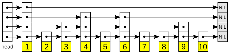
Introduction to Information Retrieval suggests about √P evenly spaced pointers for a list of length P; Lucene ties its skips to its packed blocks, since a block is decoded whole anyway. The script below runs the plain walk from 5.1 and a skipping version on trail running, counting every posting or skip entry each one looks at. The skipping version takes each doc ID from the short list and advances the long list to it.
import random

def merge(a, b):
    """Walk both sorted lists together, counting every posting we look at."""
    i = j = looked = 0
    out = []
    while i < len(a) and j < len(b):
        looked += 1
        if a[i] == b[j]:
            out.append(a[i]); i += 1; j += 1
        elif a[i] < b[j]:
            i += 1
        else:
            j += 1
    return out, looked

def with_skips(short, long, block=256):
    """For each id in the short list, jump the long list forward a whole
    block at a time using its skip entries (the last id of each block),
    then look inside one block."""
    skips = long[block - 1::block]
    b = looked = 0
    out = []
    for d in short:
        while b < len(skips) and skips[b] < d:
            b += 1; looked += 1                  # read one skip entry
        for x in long[b * block:(b + 1) * block]:
            looked += 1
            if x >= d:
                if x == d:
                    out.append(d)
                break
    return out, looked

random.seed(62)
N = 10_000_000
trail = sorted(random.sample(range(N), 1_000))       # a rare term
run = sorted(random.sample(range(N), 2_000_000))     # a common term

m, looked_merge = merge(trail, run)
s, looked_skip = with_skips(trail, run)
assert m == s
print(f"both terms: {len(m)} docs")
print(f"merge walk: looked at {looked_merge:>9,} postings")
print(f"with skips: looked at {looked_skip:>9,} postings")both terms: 202 docs
merge walk: looked at 2,000,615 postings
with skips: looked at 133,007 postingsBoth find the same 202 products. The merge walk reads all two million postings of run; with skips it looks at about 133,000, fifteen times fewer, most of them scans inside a block. A real engine does better still, decoding each block in one tight loop and crossing long stretches with its second level of skips.
We can now find every match quickly. But with the OR that search boxes use, a big shop has hundreds of thousands of matches for running shoes, and the waterproof jacket matches just as much as the road running shoe. Something has to decide which ten come first.
06Ranking: from TF-IDF to BM25
6.1What makes a match good
Why should product 3 beat product 2 for running shoes? Four ideas suggest themselves:
- Matching more of the query is better. Product 3 contains
runandshoe; product 2 onlyrun. - Rare words are worth more.
runis in four of six products, so matching it says little;shoeis in two. - Repetition counts for something. A description that says waterproof five times is probably more about it.
- Short documents are more focused. One word of four in a title matters more than one word in 2,000.
The first comes free if we add up a score per query term. The others need document frequency, term frequency and document length, all of which the index already stores.
6.2TF-IDF
A classic recipe gives each matching term a weight of its term frequency times its rarity, and adds the weights. Rarity is the inverse document frequency, IDF: the logarithm of N / df, where N is the number of documents. A term in every document gets log(1) = 0, and rarer terms get more; the logarithm stops a term in one document out of a million from outweighing everything by a factor of a million. Multiplying the two gives TF-IDF. Here IDF(run) is ln(6/4), about 0.41, and IDF(shoe) is ln(6/2), about 1.10, so product 3 scores about 1.5 and product 2 scores 0.41.
TF-IDF has two problems. The score grows in a straight line with term frequency, so a listing titled "Shoes shoes shoes running shoes shoes" scores five times as much for shoe as an honest one, when after a mention or two more repetitions should add less and less. And nothing accounts for length, so a long description gets the same credit per mention as a short, focused title.
6.3BM25
Almost every text search engine today uses a function that fixes both. It came out of the Okapi system at City University London in the early 1990s, where Stephen Robertson, Steve Walker and colleagues built it on the probabilistic model Robertson had developed with Karen Spärck Jones in the 1970s. It's called BM25, "Best Match" number 25, and Robertson and Hugo Zaragoza's 2009 survey, The Probabilistic Relevance Framework: BM25 and Beyond, is the standard account of it. For each query term t in document d, it adds:
                      tf · (k1 + 1)
score(t, d) = IDF(t) · ─────────────────────────────────
                      tf + k1 · (1 − b + b · dl / avgdl)
Here tf is the term's frequency in d, dl is d's length in terms, and avgdl is the average length. Each constant fixes one of TF-IDF's problems.
k1 controls saturation. With dl equal to avgdl and the usual k1 = 1.2, one occurrence gives 1.0, two give 1.375, five give 1.77, ten give 1.96, and nothing can push past k1 + 1 = 2.2. The seller's five shoes earn less than twice what one does.
b controls length normalisation. The bottom of the fraction grows with dl / avgdl, so a term counts for less in a longer-than-average document. b = 0 ignores length, b = 1 scales fully by it, and the usual value is 0.75.
Two products each contain 'shoe' once, and the rest of the query matches neither. Product A's title is 4 terms long; product B's description is 40 terms long; the average is 10. Using BM25 with k1 = 1.2 and b = 0.75, which ranks higher?
Lucene switched its default from a TF-IDF variant to BM25 in version 6.0, in 2016, with the textbook defaults:
public BM25Similarity() {
  this(1.2f, 0.75f, true);
}

/** Implemented as <code>log(1 + (docCount - docFreq + 0.5)/(docFreq + 0.5))</code>. */
protected float idf(long docFreq, long docCount) {
  return (float) Math.log(1 + (docCount - docFreq + 0.5D) / (docFreq + 0.5D));
}
The IDF is a smoothed log(N / df), and the 1 + inside it matters, as the next experiment shows. Lucene also drops the (k1 + 1) on top, a constant factor that can't change the order, and stores each document's length rounded into a single byte.
6.4Scoring our catalogue
SQLite's FTS5 can also rank with BM25: its bm25() function returns the score, negated so that ascending order puts the best first. This script indexes the six titles in FTS5, reads the term counts back with fts5vocab, computes BM25 by hand with k1 = 1.2 and b = 0.75, and prints its scores next to SQLite's. FTS5 keeps stop words, so the stray s counts towards product 1's length. Its last column uses Lucene's IDF instead.
import math, sqlite3
from collections import Counter

products = ["Men's trail running shoes", "Waterproof running jacket",
            "Lightweight road running shoe", "Hiking boots, waterproof leather",
            "Running socks, 3 pairs", "Aluminium snowshoes"]
db = sqlite3.connect(":memory:")
db.execute("create virtual table p using fts5(t, tokenize='porter unicode61')")
db.execute("create virtual table v using fts5vocab(p, 'instance')")
db.executemany("insert into p(t) values (?)", [(t,) for t in products])

# Read the index back: each doc's terms, then the statistics BM25 needs
docs = {}
for term, doc in db.execute("select term, doc from v"):
    docs.setdefault(doc, Counter())[term] += 1
N = len(docs)
avgdl = sum(sum(c.values()) for c in docs.values()) / N
df = Counter(t for c in docs.values() for t in c)
k1, b = 1.2, 0.75

def idf_classic(t):  # Robertson-Sparck Jones; SQLite clamps it above zero
    return max(math.log((N - df[t] + 0.5) / (df[t] + 0.5)), 1e-6)
def idf_lucene(t):   # Lucene adds 1 inside the log so it never goes negative
    return math.log(1 + (N - df[t] + 0.5) / (df[t] + 0.5))

def bm25(doc, query, idf):
    tf, dl = docs[doc], sum(docs[doc].values())
    return sum(idf(t) * tf[t] * (k1 + 1) / (tf[t] + k1 * (1 - b + b * dl / avgdl))
               for t in query if t in tf)

print(f"N={N} avgdl={avgdl:.2f} df(run)={df['run']} df(shoe)={df['shoe']}")
print(f"idf(run): classic {idf_classic('run'):.6f}  lucene {idf_lucene('run'):.3f}")
print(f"idf(shoe): classic {idf_classic('shoe'):.3f}  lucene {idf_lucene('shoe'):.3f}\n")
sqlite = dict(db.execute("select rowid, -bm25(p) from p where p match 'running OR shoes'"))
print("doc  title                          ours     sqlite   lucene-idf")
for d in sorted(sqlite, key=sqlite.get, reverse=True):
    q = ["run", "shoe"]
    print(f"{d:>3}  {products[d - 1]:30} {bm25(d, q, idf_classic):.4f}   "
f"{sqlite[d]:.4f} {bm25(d, q, idf_lucene):.4f}")N=6 avgdl=3.67 df(run)=4 df(shoe)=2
idf(run): classic 0.000001 lucene 0.442
idf(shoe): classic 0.588 lucene 1.030
doc title ours sqlite lucene-idf
3 Lightweight road running shoe 0.5667 0.5667 1.4187
1 Men's trail running shoes 0.5117 0.5117 1.2809
2 Waterproof running jacket 0.0000 0.0000 0.4773
5 Running socks, 3 pairs 0.0000 0.0000 0.4260The hand calculation and SQLite agree to four decimal places. Both shoes come first, and product 3 edges out product 1 because its title is shorter, four terms against five.
Those zeros come from the IDF. The classic IDF, ln((N − df + 0.5) / (df + 0.5)), goes negative when a term is in more than half the documents, as run is here. A negative weight would make containing run count against a product, so SQLite clamps it to almost nothing, and the jacket and socks tie at zero. Lucene's 1 + keeps the IDF positive: run still counts a little, and the shorter jacket ranks above the socks. In a real shop few query terms are in more than half the products, so the two rank almost the same.
We have a score for every matching product. The trouble is that "every matching product" can be hundreds of thousands, and the shopper sees ten.
07Finding the top ten without scoring everything
7.1Keeping only the best ten
A straightforward plan scores every doc containing any query term and keeps the best ten in a min-heap, a small structure that always knows its lowest score; each new doc that beats that score replaces it. The lowest score in the heap is the bar to clear, the threshold, θ. For trail running shoes that means scoring every product containing run, more than a million, to show ten, though most contain only run and never had a chance.
7.2WAND
At indexing time the engine can record, for each term, the highest score it contributes to any document, its upper bound. If run's upper bound is 0.8, a product containing only run scores at most 0.8, so once θ is above 0.8 none of them can get in. Broder, Carmel, Herscovici, Soffer and Zien turned that into an algorithm in 2003, WAND ("weak AND"). Here's one step on trail running shoes, with made-up numbers: upper bounds of 3.1 for trail, 1.9 for shoe and 0.8 for run, and θ = 3.5.
- Sort the three cursors by the doc they currently point at. Say
runis at doc 120,shoeat doc 410 andtrailat doc 977. - Add up upper bounds in that order until the total beats θ.
runalone gives 0.8. Addingshoegives 2.7, still not above 3.5. Addingtrailgives 5.8, which is. The doc where that happened, 977, is the pivot. - Any doc before 977 can contain at most
runandshoe, sincetrail's cursor is already at 977, so it can score at most 2.7. None of them can beat θ. So the engine advances therunandshoecursors straight to doc 977, using the skip pointers from section 5.3, and never scores anything in between. - If all three cursors now sit on 977, the engine scores that doc fully. If not, it sorts again and finds a new pivot.
As θ rises, the cursors on common terms jump further. The answer is exactly the top ten that scoring everything would give.
7.3Block-max WAND
A single upper bound per term is loose: shoe's 1.9 comes from its best document anywhere, and most stretches of its list have nothing that good. Ding and Suel's fix, in 2011, was to store an upper bound for every block of postings, next to its skip entry. After picking a pivot, block-max WAND checks the bounds of the blocks the pivot falls in, and if they add up to no more than θ, skips past the end of the shortest of those blocks without decoding them.
Lucene has done this since version 8.0, in 2019, storing for each block what it calls impacts, the term frequency and document length pairs that could score highest. Its WANDScorer cites both papers; for a top-level OR, recent versions mostly use a sibling algorithm, MaxScore, with the same block bounds.
This script compares exhaustive search, WAND and block-max WAND (blocks of 128) on a million made-up products and three terms in 5,000, 30,000 and 100,000 of them, with random title lengths and term frequencies, scored with Lucene's BM25. It counts documents fully scored and checks the top tens agree.
import bisect, heapq, math, random

random.seed(62)
N, k, BLOCK = 1_000_000, 10, 128
length = [random.randint(3, 30) for _ in range(N)]          # words per title
avgdl = sum(length) / N

def postings(df):
    """A term's postings: sorted doc ids, each with a term frequency."""
    ids = sorted(random.sample(range(N), df))
    return ids, [1 + int(random.expovariate(1.5)) for _ in ids]

def bm25(tf, dl, df):                     # Lucene's form, k1=1.2 b=0.75
    idf = math.log(1 + (N - df + 0.5) / (df + 0.5))
    return idf * tf / (tf + 1.2 * (1 - 0.75 + 0.75 * dl / avgdl))

class Term:
    def __init__(self, df):
        self.ids, tfs = postings(df)
        self.s = [bm25(tf, length[d], df) for d, tf in zip(self.ids, tfs)]
        self.ub = max(self.s)                                 # max score over the list
        self.block_last = self.ids[BLOCK - 1::BLOCK] + [self.ids[-1]]
        self.block_max = [max(self.s[i:i + BLOCK]) for i in range(0, df, BLOCK)]
        self.i = 0
    def doc(self):
        return self.ids[self.i] if self.i < len(self.ids) else N
    def advance(self, target):                                # first posting >= target
        self.i = bisect.bisect_left(self.ids, target, self.i)
    def block(self, target):              # (max score, last doc) of the block holding target
        b = bisect.bisect_left(self.block_last, target)
        return (self.block_max[b], self.block_last[b]) if b < len(self.block_max) else (0.0, N)

def search(terms, mode):
    for t in terms: t.i = 0
    top, scored = [], 0                  # min-heap of (score, doc), docs fully scored
    while True:
        theta = top[0][0] if len(top) == k else 0.0
        if mode == "exhaustive":
            d = min(t.doc() for t in terms)
            if d == N: break
        else:
            terms.sort(key=Term.doc)
            acc, p = 0.0, None
            for j, t in enumerate(terms):                     # find the pivot
                acc += t.ub
                if acc > theta: p = j; break
            if p is None or terms[p].doc() == N: break
            d = terms[p].doc()
            while p + 1 < len(terms) and terms[p + 1].doc() == d: p += 1
            if mode == "block-max":
                blocks = [t.block(d) for t in terms[:p + 1]]
                if sum(m for m, _ in blocks) <= theta:        # these blocks can't compete
                    nxt = min(last for _, last in blocks) + 1
                    if p + 1 < len(terms): nxt = min(nxt, terms[p + 1].doc())
                    max(terms[:p + 1], key=lambda t: t.ub).advance(nxt)
                    continue
            if terms[0].doc() != d:                           # skip the lists behind the pivot
                for t in terms[:p]: t.advance(d)
                continue
        score = 0.0
        for t in terms:
            if t.doc() == d:
                score += t.s[t.i]; t.i += 1
        scored += 1
        if len(top) < k: heapq.heappush(top, (score, d))
        elif score > top[0][0]: heapq.heapreplace(top, (score, d))
    return sorted(top, reverse=True), scored

terms = [Term(5_000), Term(30_000), Term(100_000)]          # trail, shoe, running
results = {m: search(terms, m) for m in ("exhaustive", "WAND", "block-max")}
best = [d for _, d in results["exhaustive"][0]]
for m, (top, scored) in results.items():
    print(f"{m:10}  fully scored {scored:>7,} docs   "
f"same top 10: {[d for _, d in top] == best}")exhaustive fully scored 131,414 docs same top 10: True
WAND fully scored 1,265 docs same top 10: True
block-max fully scored 945 docs same top 10: TrueExhaustive search scores all 131,414 matching products. WAND finds the identical top ten after scoring 1,265, about a hundredth as many, and block-max WAND after 945. The extra gain is modest here because the made-up products are scattered at random, so every block looks alike. In real collections similar documents often sit together in doc ID order, block maxima vary much more, and that's where Ding and Suel measured their large speedups.
7.4The price: no exact count
If the engine never looks at most matches, it doesn't know how many there are. Elasticsearch and OpenSearch count exactly up to track_total_hits, 10,000 by default, and then report "at least 10,000". That's why the shop in the opening said "thousands more" without a number.
Everything so far assumed the index was built once. The shop adds products every minute, changes prices, and sells out of things.
08Keeping the index fresh: segments
8.1Why the index can't be edited in place
On Tuesday morning a new product arrives, "Gore-Tex trail trainers", product 7, and the waterproof running jacket, product 2, is discontinued. Adding product 7 looks easy, since its doc ID is the largest. Removing product 2 is hard. Doc 2 is a posting inside run's, waterproof's and jacket's lists, stored as packed blocks of gaps. Taking it out changes the gap after it, which can change the whole block's bit width and size, which moves everything after it in the file. Editing a compressed index in place means rewriting most of it.
Chapter 18 met the same problem. A B+tree edits pages in place; an LSM tree never does: it collects writes in memory, writes them out as a sorted file that's never modified, and merges files in the background. Lucene arrived at the same design for inverted indexes.
8.2Segments
Lucene collects new documents in an in-memory buffer, then writes them out as a complete, self-contained inverted index of just those documents, with its own term dictionary, postings, and doc IDs starting from 0. That small index is a segment, and once written it never changes. A Lucene index is a collection of segments; a search runs against each and combines the results, adding each segment's base (the number of documents before it) to its local doc IDs. So product 7 never touches the existing postings: it goes into the buffer, and from there into a new segment.
?Isn't searching many segments slower than searching one?
Yes. A query over twenty segments does twenty dictionary lookups per term and walks twenty sets of postings. That's why segments get merged, which 8.5 comes to.
8.3Refresh: searchable within a second
Writing a segment durably means calling fsync on its files, and chapter 8 showed that fsync waits for the device. But a segment doesn't have to be durable to be searchable: Lucene can write its files into the operating system's page cache and open them for search straight away. That's a refresh, and because new documents become visible a moment after they're added, it's called near-real-time search. Elasticsearch and OpenSearch refresh once a second by default (and pause for shards that haven't been searched for 30 seconds), so product 7 shows up about a second after it's added.
A segment only in the page cache is lost in a power cut, so both engines also append every operation to a translog, fsynced before the request is acknowledged by default, which plays the part of chapter 18's write-ahead log. Every so often a flush makes a Lucene commit, fsyncing the segments and starting a fresh translog. After a crash, the engine reopens the last commit and replays the translog.
| Step | What it does | Makes the document | Default in OpenSearch |
|---|---|---|---|
| Index request | Adds the doc to the in-memory buffer and appends it to the translog | Durable (translog fsynced) but not yet searchable | translog fsync on every request |
| Refresh | Writes the buffer as a new segment into the page cache and opens it | Searchable | every 1 s, while the shard is being searched |
| Flush | Lucene commit: fsyncs segments, starts a new translog | Durable without the translog | when the translog reaches 512 MB |
8.4Deletes are marks
Now the jacket. Its segment can't change, so each segment keeps a bitset of its live documents, written as a small .liv file beside it, and deleting a doc clears its bit. It's a tombstone, like the delete markers in chapter 18's LSM tree. Queries still find doc 2 in the postings and skip it after checking the bitset. An update, such as a price change, is a delete plus an add. Deleted docs also linger in the statistics: each segment's document frequencies still count them until a merge, so after a big re-import, IDFs briefly count each product twice.
8.5Merging
Refreshes keep making small segments, and deletes leave dead documents in old ones. To fix both, the engine merges: it combines several segments' postings into one new segment, leaves out deleted documents, then switches searches over and deletes the old files.
A merge policy decides what to merge. Lucene's default, TieredMergePolicy, merges segments of similar size together, so a document is rewritten a few times on its way into a big segment instead of at every refresh. Lucene 10.5 allows about 8 segments per tier and merges up to 10 at once (OpenSearch sets 10 and 30); both cap merged segments at 5 GB and merge to reclaim space once deleted documents pass 20%. Like compaction in chapter 18, merging writes the same data several times over in exchange for fewer, cleaner segments.
Next comes size: at some point one machine can't hold the index, or answer queries fast enough.
09Spreading the index across machines
9.1Splitting by document
A Lucene index can hold a little over two billion documents, since doc IDs are 32-bit integers, but one machine runs out of memory or CPU long before that. So the index is split across machines, and there are two ways to do it. By term, each machine holds the full postings for some terms, and a query only visits the machines holding its terms. By document, each machine holds a complete inverted index of some of the products, and every query visits every machine.
Practical engines split by document. Indexing a product then touches one machine instead of one per term; the machines holding common terms like run don't become hot spots; and AND queries intersect locally instead of shipping long postings between machines. Each piece is a shard, a complete Lucene index of its own. A hash of a product's ID picks its shard, which is why the shard count is fixed when the index is created: changing it would move every product. OpenSearch's documentation suggests shards of 10 to 50 GB.
9.2Scatter and gather
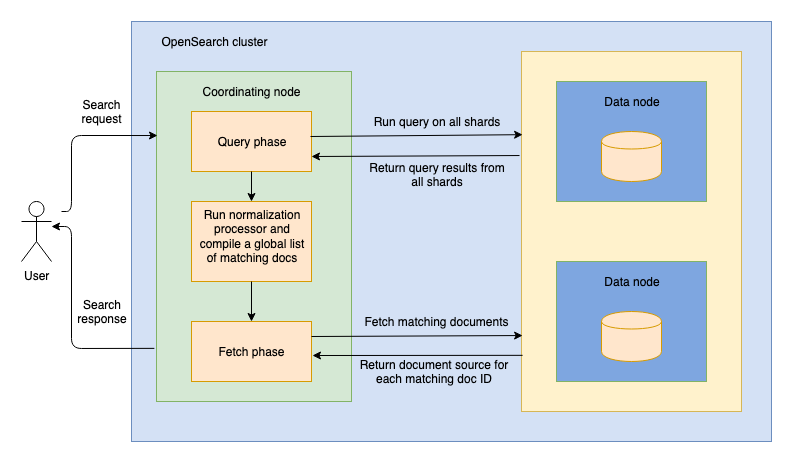
With the products split across three shards, a search goes to a coordinating node, any node in the cluster, which sends it to one copy of every shard and combines the answers. This is scatter-gather, run in two phases:
Two consequences follow. A search is as slow as its slowest shard: if one is busy merging or paused for garbage collection, every search waits, the tail-latency problem of chapter 16. And deep pages are expensive: to show results 9,991 to 10,000, the coordinator must ask every shard for its top 10,000. Both engines refuse from plus size beyond 10,000 by default (index.max_result_window) and offer search_after for walking deeper.
9.3Replicas
Each shard can have copies. The original is the primary and the copies are replicas; writes go to the primary and are passed on, and any copy can serve a search. Replicas keep shards available when a machine dies and let more searches run at once. OpenSearch creates one replica per primary by default.
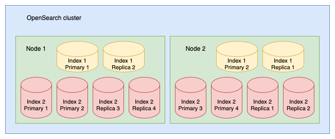
More primary shards let the index hold more products; more replicas let it answer more queries per second.
9.4Whose IDF?
There's a subtle problem in the query phase. BM25 needs each term's document frequency and the total document count, and each shard only knows its own. When products are spread at random, each shard's statistics are close to the whole index's. When they aren't, a product's score depends on which shard it landed on.
The shop routes products to shards by seller, and one seller who lists hundreds of Gore-Tex products lands on shard 2. Elsewhere, Gore-Tex products are rare. A shopper searches 'gore-tex jacket'. What happens to a Gore-Tex jacket on shard 2 compared with an equally good one on shard 0?
This is the global IDF problem. In the dfs_query_then_fetch mode, the coordinator first collects every shard's document frequencies for the query's terms and sends the totals with the query, at the cost of an extra round trip. With hash routing and reasonable shard sizes the default query_then_fetch is nearly always close enough.
So far every query has been a bag of words. Shoppers also type phrases, and they make typos.
10Phrases and typos
10.1Phrase queries
A shopper who types "trail running" in quotes wants those two words next to each other, in that order. A product titled "Running shoes for road and trail" contains both words but isn't what they mean.
Here positions earn their space. First the engine intersects trail and run as in section 5, then, for just those products, checks whether run sits exactly one position after trail. Product 1 has them at 2 and 3, so it matches. Lucene keeps positions in their own file (.pos), apart from doc IDs and frequencies (.doc), so only phrase queries pay to read them. A phrase can also allow slop: with a slop of 2, "trail shoes"~2 matches "trail running shoes".
10.2Finding terms quickly
We've treated looking up a term as instant, but a big shop's dictionary holds millions of terms, counting product codes and sellers' misspellings. Binary search would do for exact lookups, but a prefix query (water*) and a fuzzy query (10.3) need to walk terms letter by letter. The obvious structure is a trie, a tree where each edge is a letter and words with a common beginning share a path. A trie doesn't share endings, though, and endings like -ing and -proof repeat constantly. Merging every node whose remaining paths are identical turns the trie into a much smaller minimal automaton, a machine of states and labelled transitions that accepts exactly the words in the set.

A finite state transducer (FST) is such an automaton that also produces an output as you walk it, such as where a term's entry is stored on disk. Lucene used an FST as the index to its term dictionary from version 4.0 in 2012; in 10.3 it switched to a compact trie that maps a prefix to the on-disk block of 25 to 48 terms holding it. FSTs are still used for synonym tables and for autocomplete suggesters.
10.3Fuzzy queries
Now the shopper types waterprof jacket. No term waterprof exists, so we want "any term within a typo or two". The usual measure is edit distance, or Levenshtein distance: the fewest single-letter insertions, deletions and substitutions that turn one word into another. waterprof to waterproof is distance 1, and Lucene also counts swapping two neighbouring letters (watreproof) as one edit.
Computing the distance to every one of millions of terms on each keystroke is too slow. In 2002 Klaus Schulz and Stoyan Mihov showed how to build a Levenshtein automaton, which accepts exactly the strings within a given distance of a word. Lucene walks it together with the term dictionary, and as soon as a dictionary prefix can't lead to an accepted string, the whole branch is skipped: every term starting with b is ruled out after one letter. Lucene's FuzzyQuery has worked this way since 4.0, allowing at most 2 edits and expanding to the 50 closest terms by default. fuzziness: AUTO in Elasticsearch and OpenSearch allows no edits for one- or two-letter terms, one for three to five letters, and two beyond, because one edit to a two-letter word makes a different word.
All this still needs the shopper to type something close to the product's words. The next problem is the shopper who uses different words altogether.
11Hybrid search: words and meanings
11.1When the words don't match
A shopper types waterproof running shoes. Product 7, "Gore-Tex trail trainers", is exactly what they want, but it shares no term with the query, so nothing in this chapter so far will return it. This is the vocabulary mismatch problem, the limit of matching by words, which is called lexical search. Synonym lists help, but someone has to write every one.
Another approach compares meanings. A machine learning model turns text into an embedding, a list of a few hundred numbers chosen so that texts with similar meanings get similar lists, and finding similar products becomes finding the nearest points to the query's. At millions of products that needs an approximate nearest-neighbour index such as HNSW, a layered graph built on the same express-lane idea as the skip list in 5.3. Chapter 58, section 5 builds both. Lucene has had HNSW vector fields since version 9.0. This is vector search.
11.2Why run both
Vector search finds the trainers, but has its own blind spots. A shopper typing a model number, GTX-2031, wants exactly that string, and an embedding model may happily return GTX-2013; rare brands and new words the model never saw come out badly too. BM25 handles those well, because an exact rare term has a high IDF. So the common design runs both and combines the two ranked lists. That's hybrid search, and the question is how to combine them.
11.3Reciprocal rank fusion
Adding the scores doesn't work: a BM25 score has no fixed maximum and is often somewhere between 0 and 20, while a cosine similarity lies between −1 and 1, so BM25 decides everything. One fix rescales each list to 0–1 first, which OpenSearch's normalization processor has done since version 2.10. Another uses only ranks. Reciprocal rank fusion (RRF), from Gordon Cormack, Charles Clarke and Stefan Büttcher in 2009, gives each document 1 / (k + rank) from every list it's in and adds them up. With the usual k = 60, rank 1 earns 1/61 and rank 2 earns 1/62, so k stops one list's first place from dominating. 60 is still the default in Elasticsearch and in OpenSearch, which added RRF in 2.19.
This script fuses two lists for waterproof running shoes, with made-up scores of the right shapes: BM25 from the lexical index, which never finds product 7, and cosine similarities from the vector index, which ranks it first.
titles = {1: "Men's trail running shoes", 2: "Waterproof running jacket",
          3: "Lightweight road running shoe", 4: "Hiking boots, waterproof leather",
          6: "Aluminium snowshoes", 7: "Gore-Tex trail trainers"}

# query: "waterproof running shoes" -- each list is (doc, score), best first
lexical = [(1, 7.1), (3, 6.8), (2, 5.2), (4, 3.9)]               # BM25
vector  = [(7, 0.83), (1, 0.81), (4, 0.74), (3, 0.72), (6, 0.61)]  # cosine

def add_scores(*lists):
    total = {}
    for lst in lists:
        for doc, s in lst:
            total[doc] = total.get(doc, 0) + s
    return total

def rrf(*lists, k=60):
    total = {}
    for lst in lists:
        for rank, (doc, _) in enumerate(lst, start=1):
            total[doc] = total.get(doc, 0) + 1 / (k + rank)
    return total

for name, fused in [("add raw scores", add_scores(lexical, vector)),
                    ("RRF, k=60", rrf(lexical, vector))]:
    print(name)
    for doc, s in sorted(fused.items(), key=lambda x: -x[1]):
print(f" {s:8.5f} {doc} {titles[doc]}")add raw scores
7.91000 1 Men's trail running shoes
7.52000 3 Lightweight road running shoe
5.20000 2 Waterproof running jacket
4.64000 4 Hiking boots, waterproof leather
0.83000 7 Gore-Tex trail trainers
0.61000 6 Aluminium snowshoes
RRF, k=60
0.03252 1 Men's trail running shoes
0.03175 3 Lightweight road running shoe
0.03150 4 Hiking boots, waterproof leather
0.01639 7 Gore-Tex trail trainers
0.01587 2 Waterproof running jacket
0.01538 6 Aluminium snowshoesAdding raw scores reproduces the lexical order, with the trainers fifth, below a jacket, because 0.83 is tiny next to 5.2. RRF puts the two shoes first, since both lists rank them highly, then the boots, which both include, then the trainers, above the jacket.
RRF has a cost: it throws away how much better one result is than the next. Whether that matters is a question about results, and answering it needs a way to measure how good a list of results is.
12Measuring whether results are good
12.1Judgments
Every change in this chapter claims to make results better, and "better" needs a number. The standard approach is relevance judgments: sample real queries from the logs and have people grade results, say 2 for exactly right, 1 for related, 0 for irrelevant. For running shoes, products 1 and 3 get a 2, the socks a 1, everything else 0.
12.2Precision and recall
Precision is the fraction of returned results that are relevant; recall is the fraction of relevant products that were returned. Returning only product 1 gives perfect precision and poor recall; returning everything, the reverse.
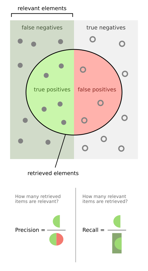
On a search page they're measured at a cutoff: precision at 10 is the relevant fraction of the top ten. Our BM25 ranking from 6.4 returned 3, 1, 2, 5: three of four are relevant, so precision at 4 is 0.75, and recall is 1.
12.3NDCG: order matters
Precision and recall ignore order: the ranking 2, 5, 1, 3, jacket first and shoes last, scores the same, though it's clearly worse. Järvelin and Kekäläinen's discounted cumulative gain (DCG), from 2002, gives each result a gain from its grade, divided by a discount that grows with rank. In the form Introduction to Information Retrieval uses, grade g at rank i contributes (2g − 1) / log2(i + 1), so a grade-2 result contributes 3 at rank 1 and 1.5 at rank 3. Dividing by the DCG of the best possible ordering gives a number from 0 to 1, NDCG.
| Rank | Ranking A (BM25) | gain | Ranking B | gain | Ideal | gain |
|---|---|---|---|---|---|---|
| 1 (÷ 1) | 3, road shoe (2) | 3.000 | 2, jacket (0) | 0.000 | 1, trail shoe (2) | 3.000 |
| 2 (÷ 1.585) | 1, trail shoe (2) | 1.893 | 5, socks (1) | 0.631 | 3, road shoe (2) | 1.893 |
| 3 (÷ 2) | 2, jacket (0) | 0.000 | 1, trail shoe (2) | 1.500 | 5, socks (1) | 0.500 |
| 4 (÷ 2.322) | 5, socks (1) | 0.431 | 3, road shoe (2) | 1.292 | 2, jacket (0) | 0.000 |
| DCG | 5.323 | 3.423 | 5.393 | |||
| NDCG | 0.987 | 0.635 | 1 |
Ranking A loses a little by putting the jacket above the socks and scores 0.987; ranking B scores 0.635 with identical precision and recall. NDCG at 10, averaged over hundreds of judged queries, is the most common single number for comparing rankers. Now we can read a claim from section 11: OpenSearch's documentation reports that on six datasets from the BEIR benchmark, RRF averaged 3.86% lower NDCG at 10 than score normalisation. It still suggests RRF as the starting point, since it works without first studying how each list's scores are spread.
12.4Offline and online
Judgments are expensive and go stale, so they serve offline evaluation, testing a change before shipping; both engines' _rank_eval API computes these metrics against your judgments. The final word comes online, from A/B tests or interleaving with real shoppers, which chapter 58 describes.
13Real systems
13.1Lucene, Elasticsearch and OpenSearch
Almost everything in this chapter runs inside one Java library. Doug Cutting wrote Lucene and first released it in 2000: analyzers, the inverted index, BM25, block-max WAND, segments, phrase and fuzzy queries, HNSW vectors, and nothing about networks. Solr and Elasticsearch wrapped it in a server and added section 9's shards, replicas and scatter-gather. Elasticsearch, first released by Shay Banon in 2010, became the most widely used. In 2021 Elastic moved it off the Apache 2.0 licence, and Amazon and others forked the last Apache-licensed version, 7.10.2, as OpenSearch, now run under the Linux Foundation. Both share the Lucene core. Here is where each idea lives:
| Idea in this chapter | Where it lives | Default |
|---|---|---|
| Analyzer (2.4) | analyzer on each text field | standard: Unicode tokenizer, lowercase, no stop words, no stemming |
| Term dictionary and index (3.1, 10.2) | Lucene .tim and .tip files | blocks of 25 to 48 terms |
| Postings, packed (4.3) | Lucene .doc (doc IDs, frequencies, skip data), .pos (positions) | packed blocks of 256 |
| BM25 (6.3) | BM25Similarity | k1 = 1.2, b = 0.75 |
| Top-k with block-max bounds (7.3) | WANDScorer, MaxScoreBulkScorer | on unless exact counts are requested |
| Exact hit count (7.4) | track_total_hits | 10,000 |
| Refresh (8.3) | index.refresh_interval | 1 s |
| Translog durability (8.3) | index.translog.durability | fsync on every request |
| Deletes (8.4) | Lucene .liv file per segment | |
| Merges (8.5) | TieredMergePolicy | 5 GB max segment, 20% deletes |
| Shards and replicas (9.1, 9.3) | number_of_shards, number_of_replicas | 1 and 1 |
| Deep paging limit (9.2) | index.max_result_window | 10,000 |
| Global IDF (9.4) | search_type=dfs_query_then_fetch | off (query_then_fetch) |
| Fuzzy queries (10.3) | fuzziness | off; at most 2 edits and 50 expansions when on |
| RRF (11.3) | OpenSearch score-ranker-processor | k = 60 |
The OpenSearch defaults are from its documentation in 2026; the Lucene ones are from the 10.5 source.
13.2Web scale: Google in 1998
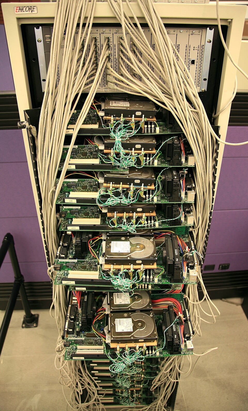
The best public account of how web search began is Sergey Brin and Larry Page's 1998 paper, The Anatomy of a Large-Scale Hypertextual Web Search Engine, from when Google was a Stanford research project. Its prototype had fetched 24 million pages, 147.8 GB, and most of this chapter is recognisable in it. Postings, which it calls doclists, were sorted by doc ID so lists could be merged quickly, the walk from section 5. Each occurrence, a hit, was packed into two bytes: a position, a rough font size and a capitalisation bit. Its full inverted index took 37.2 GB, and the lexicon, its term dictionary, held 14 million words and was kept in memory on a machine with 256 MB of RAM.
Two tricks anticipate section 7. Its index had two tiers: "short barrels" holding only hits from titles and link text, searched first, and full barrels used only if there weren't enough matches. And the searcher stopped after 40,000 matching documents, accepting slightly worse results to bound the time. Ranking combined the word-match score with PageRank, a page's importance computed from the links pointing at it. Most queries took between 1 and 10 seconds. What survived into today's engines is this chapter: sorted, compressed postings, saturating scores, and ways to avoid looking at documents that can't make the top.
14What it all costs
14.1The numbers side by side
Here are the measurements from the chapter's experiments together. The first is a timing and varies between machines; the rest are counts, and come out the same everywhere.
Each row is one idea from the chapter turning into a factor. Compression saves a factor of about six on the commonest terms; skipping saves about fifteen on a lopsided AND; top-k pruning saves about a hundred on a three-word OR. They multiply, because each applies to what's left after the one before.
14.2Why the scan never had a chance
Put the first row against the shop's real load. Say the shop has 10 million products and gets 400 searches a second at its busiest. Scanning a table costs about 40 ms per million rows, so:
| Scan time per search | 10 × ~40 ms | ~400 ms |
| Searches per second at peak | assumed | 400 |
| CPU time needed per second | 400 × 0.4 s | ~160 s |
| cores kept busy just scanning, before ranking anything | ~160 | |
And every one of those searches would still miss "shoe", return snowshoes, and come back unranked. The inverted index changes the shape of the cost: a search reads the postings of its few terms, so its work depends on how common those terms are and not on the size of the catalogue.
14.3Sizing shards and replicas
Similar arithmetic sizes a cluster. Suppose the index is split into 3 primary shards, so every search becomes 3 shard-level queries, and suppose a load test shows one copy of a shard can answer about 200 queries a second at acceptable latency. That last number is an assumption you'd measure for your own data; it depends on the queries, the hardware and how much of the index fits in memory.
| Shard-level queries per second | 400 searches × 3 shards | 1,200 |
| Copies needed of each shard for throughput | 400 ÷ 200 | 2 |
| Plus one so a node can fail at peak | 2 + 1 | 3 |
| Shard copies in the cluster | 3 shards × 3 copies | 9 |
| number_of_shards: 3, number_of_replicas: 2 | 9 copies | |
Notice that adding replicas fixed the throughput, as section 9.3 said it would. Adding primary shards wouldn't have: each search would fan out to more shards, and each shard copy would still see every search.
15Operating a search engine
15.1Where to look
Each question this chapter raised has an API that answers it on a running cluster. These are written as you'd type them in the Dev Tools console of OpenSearch Dashboards or Kibana; the same requests work with curl.
# What terms does this text become? (section 2)
GET products/_analyze
{ "field": "title", "text": "Men's trail running shoes" }

# Why did product 3 get this score? BM25 broken into its parts (section 6)
GET products/_explain/3
{ "query": { "match": { "title": "running shoes" } } }

# Where does the time go inside each shard? (sections 5 and 7)
GET products/_search
{ "profile": true, "query": { "match": { "title": "running shoes" } } }

# How many segments, how big, how many deleted docs? (section 8)
GET _cat/segments/products?v

# Which shards and replicas are where, and how big? (section 9)
GET _cat/shards/products?v

# Fewer refreshes during a bulk load (section 8.3); set it back afterwards
PUT products/_settings
{ "index": { "refresh_interval": "30s" } }

# Score a set of judged queries (section 12)
GET products/_rank_eval
{ "requests": [ ... ], "metric": { "dcg": { "k": 10, "normalize": true } } }
Reach for _explain first when a result looks wrong. It prints the IDF, term frequency, document length and average length for every query term, the pieces of the formula in 6.3.
15.2Rules that hold up
- Check your analyzer first. Many "search is broken" reports are terms analysed differently at index and query time.
- Don't ask for exact hit counts you won't show.
track_total_hits: trueturns off the skipping from section 7. - Don't refresh on every write. Let the 1-second refresh do its job, and raise the interval during bulk loads. Each forced refresh makes a tiny segment that has to be merged later.
- Force merge only indexes that are finished being written. For a live catalogue, the merge policy is better at this than you are.
- Pick the shard count at creation, aiming for 10 to 50 GB per shard, and add replicas for query volume.
- Use
search_afterfor deep paging, never largefromvalues. - Measure relevance before and after every change with a set of judged queries, and confirm with an online test.
15.3What you trade for what
| You get | You pay | When the bill arrives |
|---|---|---|
| Lookups by word, independent of catalogue size | An index built ahead of time, often larger than the text | At indexing time, and in disk space |
| Stemming that matches shoe to shoes | Overstemming: universe matches university | As odd results nobody can explain without _analyze |
| Postings at about 5 bits per doc ID | Decoding on every query; no in-place edits | When documents change, as segments and merges |
| Top 10 without scoring every match | No exact count of matches | When the product team asks for "exactly how many" |
| New documents searchable in about a second | Many small segments and constant merging | As merge I/O and slower searches during heavy indexing |
| Scale-out by sharding | Every search waits for the slowest shard; per-shard IDF | As tail latency, and rankings that differ by shard |
| Vector search finds paraphrases | A second index, a model to run, a fusion step | As memory for the vector graph and latency per query |
15.4Symptom, cause, fix
| Symptom | Likely cause | Fix |
|---|---|---|
| A product with the exact words in its title doesn't come up | Query and field analysed differently, or an exact-match term query on a text field | Compare _analyze output for both; use match for text |
| Searches for a plural miss the singular | No stemmer on the field, or a minimal one that leaves the word alone | Choose a stemmer that handles it; check with _analyze |
| Searches got slower after a big import, then recovered | Many small segments waiting to be merged | Expected; raise refresh_interval during bulk loads |
| Disk usage grows though the product count is flat | Updates leave deleted docs in old segments | Let merges reclaim them; check deleted counts in _cat/segments |
| The same product ranks differently on reload | Replicas or shards with different statistics (deleted docs, uneven routing) | dfs_query_then_fetch for small indexes; route products evenly |
| Page 1 is fast, page 500 is very slow or rejected | Each shard returns from + size results | search_after; cap pagination |
| p99 latency much worse than the median | One slow shard holds up every search | Find the slow node (merges, GC, hot shard); add replicas |
| Hybrid results look like lexical results with vectors tacked on | Raw scores added together | Normalise scores or use RRF |
16Summary
LIKE '%…%'scans every row and matches characters, not words. It misses plurals and reorderings, matches snowshoes, ranks nothing, and its cost grows with the table.- An analyzer turns text into terms: split, lowercase, perhaps drop stop words, stem. Documents and queries must go through the same one.
- An inverted index maps each term to a sorted postings list of doc IDs, with term frequencies and positions, so a search reads only the lists of its own terms.
- Postings are stored as gaps and packed in blocks, which shrank a common term's doc IDs from 32 bits each to about 5, and keeps them fast to decode.
- AND is a walk over sorted lists, and skip pointers make it as cheap as its rarest term: about 133,000 postings looked at instead of two million.
- BM25 ranks by rare terms, saturating repetition and shorter documents, with k1 = 1.2 and b = 0.75 in Lucene. Our hand calculation matched SQLite's to four decimals.
- WAND and block-max WAND find the exact top ten while skipping what can't compete: 945 documents scored instead of 131,414. The price is an approximate hit count.
- A Lucene index is a set of immutable segments, like an LSM tree's files. Refresh makes new documents searchable in about a second, deletes are bits in a live-docs file, and merges reclaim the space.
- Search scales out by splitting documents into shards and copying them as replicas. Every search fans out to every shard, waits for the slowest, and scores with each shard's own IDF unless asked not to.
- Phrases use positions, and typos use Levenshtein automata walked together with the term dictionary.
- Hybrid search runs lexical and vector retrieval and fuses the ranked lists, for example with reciprocal rank fusion, and NDCG on judged queries is how you know whether any change helped.
17Build this
A search engine for a real product catalogue, in a weekend.
- Take a few hundred thousand product titles (open product datasets are easy to find) and build an inverted index in memory: an analyzer with lowercasing and a stemmer, postings with frequencies and positions.
- Store postings as gaps in variable-byte, then in packed blocks of 128 or 256. Measure bits per doc ID for common and rare terms and compare with section 4.
- Implement BM25 and check your scores against SQLite FTS5's
bm25()on the same data, the way section 6.4 does. - Add WAND, then block-max WAND, and count documents scored for two- and three-word queries. Try sorting the products by category before assigning doc IDs and see what happens to block-max WAND's count.
- Make it accept new products into a buffer that's flushed as a new segment, support deletes with a bitset, and write a merge.
- Judge 20 queries by hand, compute NDCG at 10, and use it to choose between two stemmers.
18Interview questions
beginnerWhy can't you build product search with SQL LIKE?›
LIKE '%shoes%' can't use a B+tree index, because the pattern doesn't say how the string starts, so the database reads every row: hundreds of milliseconds at ten million rows. It's also wrong: it matches characters, so it misses shoe, misses reordered words, matches snowshoes, and doesn't rank. Search needs an index organised by word, plus analysis and ranking.
beginnerWhat is an inverted index, and what's in a posting?›
A map from each term to the list of documents that contain it, the reverse of a table that maps documents to their words. The term dictionary holds the sorted terms, each with its document frequency; each term points to its postings list. A posting holds a doc ID, a small dense integer, and usually the term's frequency in that document and its positions. Lists are sorted by doc ID, which makes them compressible as gaps and lets queries intersect them in one pass.
intermediateHow does BM25 improve on TF-IDF?›
TF-IDF grows linearly with term frequency and ignores document length, so repeating a word, or being long, inflates the score. BM25 keeps the IDF idea but passes term frequency through a saturating function controlled by k1, so the first occurrence counts most and the contribution can never exceed k1 + 1, and it normalises by document length relative to the average, controlled by b. Lucene uses k1 = 1.2 and b = 0.75, and an IDF of log(1 + (N − df + 0.5)/(df + 0.5)), which stays positive even for terms in more than half the documents.
intermediateWhy are Lucene segments immutable, and how are updates and deletes handled?›
Postings are compressed, packed blocks of gaps, so removing or inserting a posting in the middle would mean rewriting much of the file. Like an LSM tree, Lucene buffers new documents in memory and writes them as a new self-contained segment, which is never modified. A delete clears a bit in the segment's live-docs bitset, a tombstone that queries check before scoring. An update is a delete plus an add. A background merge policy combines segments of similar size, dropping deleted documents, at the cost of rewriting data several times, the same write amplification as LSM compaction.
intermediateHow does a search run across shards, and what is the global IDF problem?›
The index is split by document, so each shard is a complete index of some documents. A coordinating node sends the query to one copy of every shard; each returns only its top doc IDs and scores; the coordinator merges them and then fetches the stored data for the final page. Each shard computes BM25's IDF from its own document counts, so if a term is unevenly spread, the same document scores differently depending on its shard. dfs_query_then_fetch adds a round trip to gather global statistics first. With hash routing and decent shard sizes the default is usually close enough.
deepHow does WAND return the exact top k without scoring every match?›
Each term has an upper bound, the highest score it contributes to any document. The engine keeps a min-heap of the best k so far, whose lowest score is the threshold θ. It sorts the term cursors by current doc ID and adds their upper bounds in that order until the sum exceeds θ; the doc where that happens is the pivot. Any doc before the pivot can only contain the terms before it, whose bounds sum to at most θ, so the engine advances those cursors straight to the pivot using skip data. Block-max WAND stores a bound per block of postings and checks those too, which skips whole blocks. The result is identical to exhaustive scoring; the cost is that the total match count is only approximate.
deepHow would you combine keyword search and vector search?›
Run both: BM25 over the inverted index for exact and rare terms, and an approximate nearest-neighbour search over embeddings for paraphrases and vocabulary mismatch. Their scores aren't comparable, so don't add them. Either normalise each list's scores to a common range and take a weighted combination, or use reciprocal rank fusion, which gives each document the sum of 1/(k + rank) over the lists it appears in, with k = 60 by default. RRF needs no tuning but discards score margins; OpenSearch reports it averaged 3.86% lower NDCG at 10 than score normalisation on six BEIR datasets. Decide with judged queries and an online test.
deepCompare variable-byte and frame-of-reference compression for postings.›
Both store gaps between sorted doc IDs. Variable-byte uses 7 data bits per byte plus a flag bit, so it never goes below 8 bits per gap. Frame of reference packs a block of gaps (256 in Lucene) at the width of the block's largest gap, which took a common term to about 5.3 bits and decodes with branch-free loops. One large gap inflates its whole block, which patched frame of reference fixes by storing exceptions separately.
19Go deeper
A product title is indexed with a Porter stemmer, and a query uses Elasticsearch's term query for 'shoes'. Why does it find nothing?›
The index holds the term shoe. A term query skips analysis, so it looks
up shoes exactly, and no such term exists. A match query would analyse
the query with the field's analyzer first.
Why does an AND of a rare word and a very common word cost about the same as the rare word alone?›
The engine leads with the short list and uses skip data to jump the long list forward to each of its doc IDs, decoding only the blocks that could contain them.
You deleted 30% of the products, and disk usage didn't go down. Why?›
Deletes only clear bits in each segment's live-docs file. The postings stay until merges rewrite the segments without the deleted documents.
Why does the classic BM25 IDF give zero weight to a term in four of six documents?›
ln((N − df + 0.5)/(df + 0.5)) is negative when df is more than half of N, and implementations like SQLite clamp it to almost zero. Lucene adds 1 inside the logarithm to keep it positive.
The textbook for this chapter: Boolean retrieval and skip pointers (chapters 1–2), index compression (chapter 5), scoring (chapters 6 and 11) and evaluation (chapter 8). Free online from Stanford's NLP group.
Where BM25 comes from, what k1 and b mean in the model, and its extension to documents with several fields.
The WAND paper: upper bounds, pivots, and the two-level evaluation that skips documents which can't make the top k.
Per-block score bounds, and the block-max WAND algorithm Lucene adopted in version 8.0.
Google as a Stanford prototype: hit lists, barrels, the lexicon, PageRank, and the storage statistics quoted in section 13.2.
Two pages that introduced RRF and the constant k = 60 that engines still use as their default.
How to build an automaton that accepts every string within n edits of a word, the basis of Lucene's fuzzy queries.
The package documentation in the Lucene source describes every file in a segment: the term dictionary, packed postings, skip data and impacts.
20Related chapters
LSM trees, memtables, immutable files, tombstones and compaction: the
design Lucene's segments and merges follow, and the B+tree that can't help
LIKE '%…%'. Chapter 18.
Embeddings, and the nearest-neighbour indexes (IVF and HNSW) behind the vector half of hybrid search. Chapter 58.
Why refresh can make a segment searchable without fsync, and what the
translog's fsync costs. Chapter 08.
Hash partitioning, hot spots, and why changing the number of partitions is hard: the same issues as choosing a shard count. Chapter 29.
Why a request that fans out to many shards is held up by the slowest one. Chapter 16.