Someone tells you the /report page takes too long to load. You open the code behind it and a few places look suspicious: a database query, some string formatting, a loop that matches each order to its customer. You pick the one that looks worst and spend the afternoon making it faster. The page is exactly as slow as before.
That happens to nearly everyone, because people are bad at guessing where a program spends its time. A change made on a guess either does nothing or moves the cost somewhere harder to see. A good mechanic doesn't start replacing parts when an engine runs badly. They plug in a diagnostic reader and measure first, so the reader tells them where to look before anything gets touched.
Software has diagnostic readers too, and this chapter follows the slow /report request through them. The question we ask the whole way is: where does the time go, and how will we know our fix worked? We start by putting a profiler on the report's code, then widen out to what a real service adds: whether the request is even running code, which machine to look at, which lines burn the CPU, and how to time a change without being fooled by the measurement itself.
01Finding where the report spends its time
1.1Profiling the report's code
Let's make the report concrete. It matches 6,000 orders to 3,000 customers, so that each order can be printed with its customer's name. The first version, slow_report, does what most of us would write first: for each order, walk down the customer list until the right customer turns up. A second version, fast_report, builds a dictionary from customer id to name once, and then looks each order up in it.
Python ships with a profiler called cProfile. A profiler is a tool that watches a program run and records how much time each function took. We'll profile slow_report alone and print the two functions with the most self time, meaning time spent in a function's own lines and not in the functions it calls. After that the script times both versions with time.perf_counter(), a stopwatch, to see how much faster the second one is. Save it as prof.py and run it with python3 prof.py.
import cProfile, pstats, time

def slow_report(orders, customers):
    result = []
    for o in orders:
        for c in customers:                     # scans the whole customer list for every order
            if c["id"] == o["customer_id"]:
                result.append((o["id"], c["name"]))
                break
    return result

def fast_report(orders, customers):
    by_id = {c["id"]: c["name"] for c in customers}      # build a lookup once
    return [(o["id"], by_id[o["customer_id"]]) for o in orders]

orders    = [{"id": i, "customer_id": i % 3000} for i in range(6000)]
customers = [{"id": i, "name": f"c{i}"} for i in range(3000)]

pr = cProfile.Profile(); pr.enable(); slow_report(orders, customers); pr.disable()
stats = pstats.Stats(pr)
total = sum(tt for (_, _, tt, _, _) in stats.stats.values())
print("where the time went (self time, from the profiler):")
for (file, line, name), (cc, nc, tt, ct, callers) in sorted(stats.stats.items(), key=lambda kv: -kv[1][2])[:2]:
    print(f"  {name:<32} {tt:6.3f} s  {tt / total:6.1%}")

t = time.perf_counter(); slow_report(orders, customers); slow = time.perf_counter() - t
t = time.perf_counter(); fast_report(orders, customers); fast = time.perf_counter() - t
print(f"\nslow_report: {slow:.3f} s fast_report: {fast:.4f} s ({slow / fast:,.0f}x faster)")where the time went (self time, from the profiler):
slow_report 0.164 s 99.8%
<method 'append' of 'list' objects> 0.000 s 0.2%
slow_report: 0.164 s fast_report: 0.0004 s (449x faster)Read the first two output lines. The profiler put 99.8% of the time inside slow_report itself, and almost none in append, the list method that stores each result. The report spends its time in its own loop and nowhere else. The last line shows what fixing that one loop is worth: in the run above the dictionary version was about 449 times faster, and another run gave 463. The exact ratio changes from run to run and from machine to machine, but it stays in the hundreds.
1.2What the measurement saved us from
Nothing in that output pointed at append, at the string formatting, or at the amount of data. The time was in the loop that scans customers for every order, and a guess might have started anywhere else. Counting shows why the loop costs so much. The orders' customer ids cycle through 0 to 2,999, so the scan walks about 1,500 customers on average before it finds a match. Across 6,000 orders that makes about 9 million comparisons, each one executed by the Python interpreter. The dictionary version does 3,000 insertions and 6,000 lookups, about a thousand times fewer steps.
The pattern for everything that follows is already visible here: measure first, let the numbers choose the target, change one thing, and measure again.
This was a friendly case, though. The slow code was one Python function that kept a core busy the whole time, and we already knew which function to profile. A real /report request passes through a web server, a database and a network, on one of many machines, and a profiler attached to one program sees only a slice of that. Before reaching for more tools we need to say precisely what we're trying to improve.
02Deciding what faster means
2.1Three different goals
In the experiment, better meant that the report finished sooner. For a real service, "make /report faster" can mean three different things, and they pull in different directions.
The first is latency, the time one request takes from the moment it arrives to the moment its answer leaves. We describe latency with percentiles. The p50 is the time that half of all requests beat, so it describes the typical request. The p99 is the time that 99 of every 100 requests beat, so it describes the slowest 1%. Users feel the slow end, which is why teams watch p99. The second goal is throughput, how many requests the service finishes per second. The third is efficiency, how much hardware each request costs.
| Goal | The question | Typical unit | What usually improves it |
|---|---|---|---|
| Latency | How long does one request take? | ms at p50, p99 | Less work per request, less waiting |
| Throughput | How many requests per second at an acceptable latency? | req/s at a latency target | More work in parallel, less waiting for shared locks |
| Efficiency | How much hardware does each request cost? | CPU-seconds or dollars per million requests | Less work per request |
Batching shows the pull between them. Suppose /report saved up ten requests and answered them with one database query. Throughput and efficiency go up, because the fixed cost of a query is paid once for ten requests. Latency goes up too, because the first request of each batch now sits waiting for the other nine to arrive.
?Why write the goal down?
Because it decides what "better" means when you measure. A change that halves CPU per request but adds a millisecond of queueing is a win for the cloud bill and a loss for the p99. If you haven't decided which one you're after, you'll report whichever number moved the right way.
2.2How much a fix can be worth
Say the goal is /report's latency, and a profile has shown that one function owns 10% of each request. How much faster does the request get if we make that function twice as fast? The arithmetic is called Amdahl's law. If a part of the work takes a fraction p of the total and we make it s times faster, the whole thing speeds up by:
speedup = 1 / ((1 − p) + p / s)A function takes 10% of a request's time. You rewrite it to be twice as fast. How much faster is the request?
Now try a bigger slice. A function that owns 40% of the request, made twice as fast, gives 1 / (0.6 + 0.4 / 2), which is 1 / 0.8, a 25% speedup. It's the same fix as before with five times the payoff, purely because the slice it works on is four times bigger.
Amdahl's law talks about the share of a request's time that a function owns. But a share of what? A request's time isn't all spent running code, and that changes which tool can see it.
03Running or waiting
3.1Two kinds of time
Picture one /report request from the moment it arrives. A thread in the web server picks it up, and that thread can only run instructions while it sits on a core, one of the CPU's independent processors. A machine usually has more threads than cores, so they take turns. The kernel, the part of the operating system that manages the hardware, decides whose turn it is, and the piece of the kernel that does this is called the scheduler. Threads that are ready to run but have no free core wait in a line called the run queue.
Now hold two stopwatches over this request. The first is the wall clock, what a stopwatch in your hand would show from arrival to answer. The second is CPU time, which only ticks while the request's thread is running on a core. We'll call the time it spends running on a core on-CPU, and all the rest off-CPU. The scene follows the thread through one request.
/report request arrives and a thread starts parsing it on a core. Both clocks tick: the wall clock always does, and CPU time ticks while the thread runs.Off-CPU covers every reason a thread isn't running: blocked on a lock, a disk read, a network reply or a free slot in a pool of connections (a pool is a fixed set of reusable workers or connections that requests have to wait for), or ready and waiting in the run queue. This request spent 5 ms on-CPU and 195 ms off.
A profiler that looks at the code running on the cores sees none of those 195 ms. A blocked thread executes no instructions, so it leaves nothing to look at, and section 5 shows exactly how that kind of profiler takes its samples.
The request above took 200 ms, with 5 ms on a core. You find the code that ran on the core and make it twice as fast. Roughly how long does the request take now?
3.2Telling which kind you have
Compare CPU time to wall time for the slow requests. If a request takes 200 ms and its thread was on-CPU for 180 ms, the time is in the code, so profile the CPU. If it was on-CPU for 5 ms, the other 195 ms were spent waiting, and a CPU profile will give you a tidy picture of the 5 ms that don't matter. For a whole command, the shell's time prints both numbers: real is the wall clock, and user plus sys is CPU time.
Chapter 16 shows the extreme case. In a lock convoy, threads line up behind one lock and each spends most of its life waiting for it. There, p99 got eleven times worse while the CPU profile stayed flat, because waiting for a lock is off-CPU time.
Knowing which kind of time we're hunting helps once we know where to look. In production we don't yet: the slow /report could be one endpoint among fifty, on one of hundreds of machines, waiting on any of a dozen resources. We need a routine way to narrow that down.
04Narrowing down to a service and a resource
When a system is slow and you don't yet know why, a checklist beats intuition. It makes you look at the things you'd otherwise skip, and it's fast. Two checklists cover most of the ground, one for services and one for machines.
4.1The RED method: which endpoint is hurting
The complaint was about one page, but the service behind it has many endpoints. Tom Wilkie's RED method asks three things of every endpoint: Rate ("the number of requests per second"), Errors ("the number of those requests that are failing") and Duration ("the amount of time those requests take"). Duration is the latency from section 2, shown as percentiles.
Plot those three for /report against deploys and traffic changes, and you learn whether /report got slower, since when, and whether anything else changed at that moment. RED tells you which endpoint is hurting its users. It doesn't say why, and for that we look at the machines and pools behind it.
4.2The USE method: which resource is the bottleneck
Brendan Gregg's USE method is one sentence: "For every resource, check utilization, saturation, and errors." A resource is anything with a finite capacity: CPUs, memory, disks, network interfaces, and software resources such as a mutex (a lock that lets one thread at a time through), a thread pool or a connection pool.
| Metric | Gregg's definition | What it looks like |
|---|---|---|
| Utilisation | "the average time that the resource was busy servicing work" | CPU 70%, disk 90% busy |
| Saturation | "the degree to which the resource has extra work which it can't service, often queued" | Run-queue length, I/O queue depth, threads waiting on a pool |
| Errors | "the count of error events" | NIC drops, ECC errors, EMFILE on accept() |
The examples in the last cell are all small failures worth a look: a NIC (network interface card) dropping packets, ECC (error-correcting memory) reporting a repaired bit flip, and EMFILE, the error a program gets when it has hit its limit on open files.
?Why is saturation the one to watch?
Because utilisation is an average, and averages hide bursts. A disk that's 60% busy over a minute may have been 100% busy for twenty seconds with a queue behind it. Saturation measures that queue directly, and queueing is where latency comes from (the arithmetic is in chapter 16).
Gregg keeps a Linux checklist that maps each cell to a command. Tools such as vmstat 1 and iostat -xz 1 print a fresh line of numbers every second when you give them an interval of 1, so you watch the numbers move. The rows you'll use most:
| Resource | Utilisation | Saturation | Errors |
|---|---|---|---|
| CPU | vmstat 1: us + sy + st | vmstat 1: r above the CPU count; /proc/pressure/cpu | Rarely visible without vendor counters |
| Memory | free -m | vmstat si/so (swapping); OOM kills in dmesg | dmesg for hardware errors |
| Network | sar -n DEV 1 against link speed | Drops, overruns, retransmits (nstat) | ip -s link errors |
| Disk | iostat -xz 1 %util | iostat queue size above 1, high await | smartctl, dmesg |
| File descriptors | ls /proc/PID/fd | wc -l against the limit | n/a | EMFILE from open() and accept() |
A few of the terms: in vmstat, us is the share of CPU time spent in programs' own code, sy the share spent in the kernel on their behalf, and st ("steal") the share a virtual machine wanted but the host gave to another machine. r is the number of threads in the run queue, si/so are memory pages swapped in from disk and out to it, an OOM kill is the kernel ending a process because memory ran out, and a retransmit is a network packet that had to be sent again. /proc/pressure/* is PSI (pressure stall information, added in Linux 4.20). It reports the share of time some task was stalled waiting on CPU, memory or I/O, which is saturation measured directly.
4.3A USE pass, step by step
Here is the order in which to run the pass on one host. Each step either finds a saturated resource or rules one out in under a minute.
dmesg -T | tail, NIC drops, OOM kills. An error is usually unambiguous, and checking takes seconds.Gregg reckons the method "solves about 80% of server issues with 5% of the effort". Most of the rest need a profiler, the subject of section 5. One saturation is easy to miss with these tools, though, and it's the one containers add.
4.4The saturation nobody graphs: CPU throttling in containers
Containers, and Kubernetes pods in particular, are limited by a kernel feature called cgroups, which caps how much CPU, memory and I/O a group of processes may use. The CPU cap is a quota: an amount of CPU time the group may use in each 100 ms period. A container with a limit of 4 CPUs gets 400 ms of CPU time per 100 ms period, however many cores the host has. Suppose eight of its threads run flat out on a host with at least eight cores. Together they use up the 400 ms in 50 ms of wall time, and the kernel throttles the group, meaning it pauses every thread in it until the next period starts. For the other 50 ms every request in that container waits.
Three files in the cgroup directory show this. cpu.max holds the quota and the period in microseconds, cpu.stat holds usage and throttling counters, and cpu.pressure is the PSI view of the same container. The commands below read all three.
cat /sys/fs/cgroup/cpu.max
cat /sys/fs/cgroup/cpu.stat
cat /sys/fs/cgroup/cpu.pressure400000 100000
usage_usec 2975847350
user_usec 2014181826
system_usec 961665523
nr_periods 11985
nr_throttled 4964
throttled_usec 950837608
some avg10=20.26 avg60=16.05 avg300=17.44 total=243046491
full avg10=9.07 avg60=6.32 avg300=7.49 total=129115661The first line says 400,000 µs of CPU per 100,000 µs period, the 4-CPU limit. In cpu.stat, nr_periods counts the periods so far and nr_throttled counts those in which the container used its whole quota and was paused until the next one. Here that's 4,964 of 11,985 periods (41%), and throttled_usec says about 951 seconds were lost to it in total. The host has ten cores, so top inside the container never showed the CPUs as full. In the PSI lines, some is the share of time at least one task in the container was stalled waiting for CPU, and full is the share when every task was. avg10=20.26 means that over the last 10 seconds, some task was stalled about 20% of the time. The 60- and 300-second averages are close to it, so this has been going on for minutes and isn't a single spike.
?Why doesn't CPU utilisation show it?
Because the usual dashboards compare usage to the node's cores, or average it over a minute. A service can average 50% of its limit and still be throttled in most periods, if its work arrives in bursts that use the whole quota in the first part of each 100 ms period. Each throttle adds up to the rest of that period to every request caught in it.
Linux 5.4 fixed one kernel cause of excess throttling (de53fd7aedb1): per-CPU slices of quota were expiring unused, so "highly-threaded, non-cpu-bound applications" were throttled "while simultaneously not consuming the allocated amount of quota". The fix helps, but bursty work under a tight limit still throttles.
4.5Three questions, three tools
RED and USE look at different things. Wilkie summed up the pair like this: "The RED Method is about caring about your users and how happy they are, and the USE Method is about caring about your machines and how happy they are." Google's SRE book adds a third list, the four golden signals, which is RED with saturation attached.
| Checklist | Unit of analysis | Answers | Misses |
|---|---|---|---|
| RED | A service or endpoint | Which endpoint is slow or failing, and since when? | Why it's slow |
| USE | A resource: CPU, disk, pool, lock | Which resource is the bottleneck? | Whether users are hurting |
| Four golden signals (Google SRE) | A service | Latency, traffic, errors, and saturation | Which code is responsible |
So the order of work is RED to find which service and endpoint regressed and when, USE on the hosts and pools behind it to find which resource it's waiting on, and a profiler to find which code is burning that resource. Suppose the pass ends with the CPU saturated. We know the resource, and now we need the code, which means sampling what the CPU is doing.
05How a sampling profiler works
5.1Tracing and sampling
In section 1, cProfile found the slow loop by recording every function call and return. That makes it a tracing profiler. A tracing profiler's call counts are exact, but the recording adds work to every call, so the program runs slower under it, and functions that make many small calls look more expensive than they are. That was fine for a script that runs for a fraction of a second. On a production service the extra cost lands on every request, so people rarely leave a tracing profiler running there.
A sampling profiler takes a different route. It pauses the program briefly at a fixed rate and writes down where the program was. At 99 samples a second on one core, it wakes 99 times a second, records a stack each time (we'll define that in a moment), and otherwise leaves the program alone. Functions that run often show up in many samples and functions that run rarely show up in few, so the counts converge on the share of CPU time each function owns. On Linux the standard tool for this is perf, and knowing how it collects one sample explains most of the ways its output can mislead you.
?Why 99 Hz and not 100?
Gregg's perf examples explain it: "to avoid accidentally sampling in lockstep with some periodic activity, which would produce skewed results." Plenty of software runs on 10 ms timers, maybe including yours. Sampling at exactly 100 Hz could land on the same phase of that timer every time.
5.2One sample, from interrupt to file
To keep the example small we'll use a toy C program standing in for the /report handler. handle_request calls three phases in turn, parse, lookup and format. Each one is marked noinline, which tells the compiler to keep it as a separate function instead of folding it into its caller.
When main calls handle_request, which calls lookup, the program keeps a small record for each call in a region of memory called the call stack, and each record is a frame. If we froze the program while it ran lookup, the stack would read main, handle_request, lookup: the answer to "how did we get here?". That list is what a profiler wants for each sample.
Getting the list takes some help from the program. The CPU's registers are a handful of named storage slots inside each core. One of them, the program counter (PC), holds the address of the instruction being executed, which tells us which function we're in. The callers are harder. When a function starts, it saves two words in its frame: the address of its caller's frame, and the return address, the spot in the caller where execution resumes when the function returns. Then it points a register at that pair. This register is the frame pointer, called x29 on arm64 and rbp on x86-64. Every frame therefore links to its caller's frame, like a linked list running down the stack, and walking the stack means following the list.
The scene below shows one sample being taken, with x29 pointing into the stack.
lookup(), called by handle_request(), called by main(). The stack has one frame per call. The PC says we're in lookup, and x29 points at its frame.Notice how little a sample costs: the interrupt, then two memory reads per frame. The stack walk is the biggest part of that cost, and it is also the fragile part, because it only works if every function on the stack kept its link.
5.3The walker in the kernel
Here is the code the kernel runs for the stack walk of a user program on arm64. It's short because the frame-pointer layout is so simple.
struct frame_tail {
	struct frame_tail	__user *fp;
	unsigned long		lr;
} __attribute__((packed));

static struct frame_tail __user *
unwind_user_frame(struct frame_tail __user *tail, void *cookie,
	       stack_trace_consume_fn consume_entry)
{
	struct frame_tail buftail;
	/* ... */
	pagefault_disable();
	err = __copy_from_user_inatomic(&buftail, tail, sizeof(buftail));
	pagefault_enable();
	/* ... */
	lr = ptrauth_strip_user_insn_pac(buftail.lr);

	if (!consume_entry(cookie, lr))
		return NULL;

	/*
	 * Frame pointers should strictly progress back up the stack
	 * (towards higher addresses).
	 */
	if (tail >= buftail.fp)
		return NULL;

	return buftail.fp;
}

void arch_stack_walk_user(stack_trace_consume_fn consume_entry, void *cookie,
					const struct pt_regs *regs)
{
	/* ... */
		tail = (struct frame_tail __user *)regs->regs[29];
		while (tail && !((unsigned long)tail & 0x7))
			tail = unwind_user_frame(tail, cookie, consume_entry);
	/* ... */
}
struct frame_tail is the saved pair from the scene, fp for the caller's frame and lr for the return address. The loop at the bottom starts at x29 (regs->regs[29]), copies the two words, records the return address, and repeats until the chain stops going up the stack. The copy runs with page faults disabled. A page fault happens when a program touches memory the kernel hasn't loaded yet, and handling one can mean waiting for the disk. Code running inside an interrupt must never wait, so if a frame isn't in memory the copy fails and the walk stops there.
This only works if the program kept the links. GCC and Clang omit frame pointers at -O2 on many targets, because it frees a register for other uses. Gregg's history traces the default to a 2004 GCC change made for 32-bit x86, where the register was scarce. What does the walker do when a function never saved its link?
5.4What a broken stack does to a profile
Without a link, x29 holds whatever the function last used it for, and the walker follows it anyway. It skips frames, or reads garbage, or stops early. Here is the same sample taken in a program built without frame pointers.
lookup records the full chain: lookup, handle_request, main.To check, we can build the toy program twice with GCC 13.3 at -O2, once with -fno-omit-frame-pointer and once with -fomit-frame-pointer, and profile both. The flags in the commands: -O2 turns on optimisation, -g adds debug information, and the two -f flags choose whether frame pointers are kept. perf record -F 999 -g samples 999 times a second (-F), ten times the usual rate because the toy program only runs for a few seconds, and records call stacks (-g); -o names the output file, and the command to profile comes after --. The script collapse.py is a small helper that joins each sample's stack into one line, outermost function first, followed by a count of how many samples had that exact stack. Section 6 explains that format.
gcc -O2 -g -fno-omit-frame-pointer -o svc_fp   svc.c
gcc -O2 -g -fomit-frame-pointer    -o svc_nofp svc.c
perf record -F 999 -g -o fp.data   -- ./svc_fp 400000
perf record -F 999 -g -o nofp.data -- ./svc_nofp 400000
perf script -i fp.data | ./collapse.py | head -3
perf script -i nofp.data | ./collapse.py | head -3_start;[unknown];[unknown];main;handle_request;lookup 1281
_start;[unknown];[unknown];main;handle_request;parse 830
_start;[unknown];[unknown];main;handle_request;format;[unknown];... 169
_start;[unknown];handle_request;lookup 1439
_start;[unknown];handle_request;parse 828
_start;[unknown];format;[unknown];[unknown];[unknown];[unknown] 181The first three lines are the run with frame pointers. Each line reads left to right from the outermost function to the one that was running, with the sample count at the end. With frame pointers, all 2,458 samples had main and handle_request in their stack. The second three lines are the run without them, and there only 2 of 2,649 samples had main, while 382 samples (14%) showed format with no handle_request above it. The [unknown] frames are library code without symbols installed, which is a different problem (section 6.5).
Even the broken profile has the right leaf functions. What it gets wrong is the ancestry: format looks as if something other than handle_request called it. In a real service with fifty callers of a JSON encoder, that's the difference between "the encoder is slow" and "the encoder is slow when the audit endpoint calls it".
5.5The other ways to walk a stack
Frame pointers aren't the only way to recover the chain, and each alternative has a price. Three terms appear in the table. DWARF is the standard format for debug information, and it includes tables that say how to undo each function's changes to the stack. LBR (last branch record) is a CPU feature that logs the most recent jumps the program took. A JIT (just-in-time compiler, as in the JVM and Node.js) builds machine code while the program runs, so its code has no debug information on disk.
| Method | How it works | Cost | Where it breaks |
|---|---|---|---|
| Frame pointers | Follow saved fp/lr pairs | A few loads per frame; one register given up | Any code built without them, including some JIT and hand-written assembly |
DWARF (--call-graph dwarf) | Copy a chunk of raw stack per sample; unwind later with debug info | Large perf.data, slow post-processing | Stacks deeper than the copied chunk; JIT code has no DWARF |
LBR (--call-graph lbr, Intel) | Hardware records recent branches | Nearly free | Limited depth (tens of entries); needs hardware support, often not exposed in VMs |
| ORC | Kernel-only unwind tables generated at build time | Cheap | Kernel only |
| SFrame | A compact user-space format modelled on ORC | Cheap | Needs toolchain and kernel support, still arriving |
ORC and SFrame are the same idea as DWARF's tables in a smaller, faster form. For a profiler you want running all the time, the cost column decides, so it's worth seeing what DWARF's cost looks like.
DWARF mode on the same frame-pointer-less binary recovered main in 2,144 of 2,475 samples (87%). It paid for that in file size: perf.data was 21.2 MB against 0.32 MB for the frame-pointer run of the same length, roughly 66× larger, because each sample carries a copy of the raw stack.
?So why did distributions turn frame pointers back on?
Because the cost turned out small and the benefit large. Fedora 38 added -fno-omit-frame-pointer to its default build flags (change page), and Ubuntu 24.04 did the same for 64-bit platforms, measuring a penalty "between 1-2% in most cases" (Canonical). Gregg reports overhead at Netflix "usually less than one percent".
We now have thousands of samples, each one a stack. Nobody can read that as text, so we need a way to see the whole profile at once.
06Reading a flame graph
6.1From samples to a picture
A profile of a real service has tens of thousands of distinct stacks. Gregg invented the flame graph in 2011 while debugging MySQL, because profiler text output was a wall nobody could read (flamegraphs.html). The first step is the format you saw in section 5.4: one line per distinct stack, with the frames joined by semicolons, outermost first, then a count. Producing it is called folding the stacks. The frame-pointer profile from section 5.4, trimmed of the start-up frames above main and with every stack under each phase added together, folds to three lines:
main;handle_request;lookup   1281
main;handle_request;parse     830
main;handle_request;format    347
The scene below does the folding on ten samples of the toy handler, a number small enough to draw. In the real profile there were 2,458.
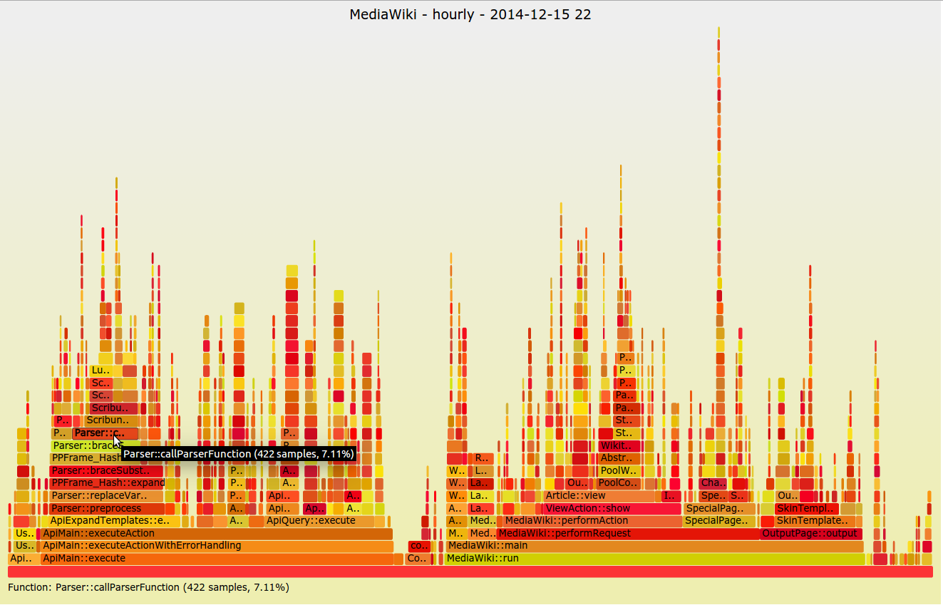
main → handle_request → that function. The number is the order the sample arrived in.The real flame graph has the same shape. handle_request is 100% wide and splits into lookup (52%), parse (34%) and format (14%), the shares of 1,281, 830 and 347 out of 2,458 samples.
?Why care about the folded format?
Because it's a universal interchange. perf, bpftrace, async-profiler for the JVM, py-spy and Go's pprof can all produce folded stacks, and once you have them you can grep, diff and sum them with shell tools. Two profiles folded the same way can be subtracted line by line, which is how the before-and-after graphs of section 6.4 are made.
6.2What the axes mean
The scene used each part of the picture in a particular way, and it's worth stating them together.
| Element | Meaning | Not |
|---|---|---|
| Box | One function in one stack | A single call |
| Width | How many samples had this frame: its share of CPU | Duration of one call |
| y-axis | Stack depth; each box's parent is its caller | Time |
| x-axis | Stacks "sorted alphabetically (it is not the passage of time)" | Time order |
| Top edge | What was on-CPU | |
| Colour | Usually random warm hues, or by type (kernel, JIT, user) | Heat or cost |
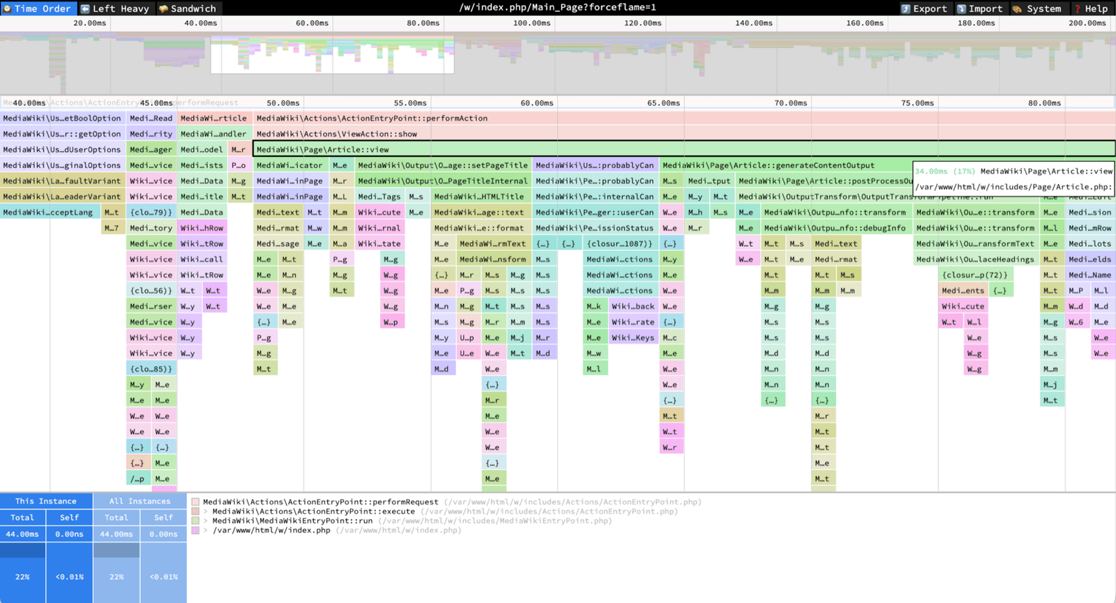
Sorting is the reason identical stacks merge. If samples were placed in time order, the same call path would appear in hundreds of thin slivers, but sorted by name every sample of main;handle_request;lookup sits together and they merge into one wide box. The price is that the x-axis carries no time information. Two boxes side by side didn't run one after the other, and for a time-ordered view you need a flame chart (Chrome DevTools and Perfetto draw them) instead, which is a different picture.
6.3How to read one in five minutes
- Find the widest towers near the top. A wide box whose children are narrow is a function doing work itself. That's your target.
- Read plateaus, not peaks. Tall thin spikes are deep call chains that run rarely. They catch the eye, but a narrow box owns few samples, so it rarely matters.
- Search. The SVG that Gregg's FlameGraph tools draw (section 11.1) is interactive and has a search box. Searching
malloc,lockormemcpyhighlights and totals every match across all stacks. - Check the ancestry of a hot leaf. The same leaf under two different parents is two different problems.
- Look for what shouldn't be there. Logging, regex compilation, exception construction, JSON re-parsing and TLS handshakes are common surprises.
6.4Off-CPU and differential flame graphs
A CPU flame graph can't answer two questions we met earlier, so there are two variants.
The first question is where the 195 ms of waiting from section 3 went. An off-CPU flame graph records a stack every time a thread blocks, weighted by how long it stayed blocked, so width becomes time spent waiting on a lock, a read or a sleep. It's collected at the scheduler's sched:sched_switch tracepoint (a hook the kernel provides at the moment it switches threads) with tools such as offcputime. These are built on eBPF, a way to run small, checked programs inside the kernel at hooks like that one (chapter 48 covers how).
The second question is what got slower in this release. A differential flame graph compares two profiles, before and after a change, and colours each frame by whether it grew or shrank. Instead of eyeballing two graphs side by side, you see the frames that changed in red and blue.
You can combine on-CPU and off-CPU into one graph, but the units differ. An on-CPU sample is CPU time on one core, and an off-CPU sample is waiting time for one thread. With 200 threads mostly idle in a pool, the off-CPU graph is dominated by idle waiting that's perfectly healthy, so filter to the threads that serve requests before reading it.
6.5Symbols: JITs, containers and stripped binaries
A symbol is the name that goes with an address in a program, and the profiler needs symbols to print lookup instead of 0x4012a8. When a flame graph is full of [unknown], the stacks are usually fine and the names are what's missing. JIT-compiled code creates its machine code while the program runs, so no file on disk holds its names.
| Symptom | Cause | Fix |
|---|---|---|
JVM frames all [unknown] or Interpreter | perf can't read JIT-compiled code's names | async-profiler, or -XX:+PreserveFramePointer plus a perf-PID.map agent |
| Node.js frames missing | Same JIT problem | node --perf-basic-prof |
Everything in a container [unknown] | perf on the host can't see the binary at the path the container used | Run perf inside the container, or use --symfs |
libc frames [unknown] | No debug symbols installed | Install the -dbg or -debuginfo package, or use a debuginfod server |
| Stacks end after one or two frames | No frame pointers | Section 5.5 |
The third row can happen the other way round too. A program profiled from inside a container produced a profile that was all [unknown], because its binary sat on a host-mounted path that perf report couldn't open from there. Copying the binary to a local path fixed every symbol.
A flame graph tells us where the cycles go. It doesn't tell us why a function needs so many of them.
07Why the CPU is slow in that function
Suppose the flame graph says lookup owns half the CPU. There are several very different ways to make it cheaper, and the right one depends on what the core is doing during those cycles. For that, the CPU's performance monitoring unit (PMU) counts events in hardware: cycles, instructions, cache misses and branch mispredictions. A cache miss means the data wasn't in the CPU's small fast cache and had to be fetched from slower memory (chapter 02). A branch misprediction means the CPU guessed wrongly which way an if would go and threw away work (chapter 01).
7.1IPC: the first number to read
perf stat runs a command and prints counter totals. Read instructions per cycle (IPC) first. It says how many instructions the core finishes, or retires, per clock tick, on average.
| IPC | What it usually means | Where to look |
|---|---|---|
| Below about 1 | The core is mostly stalled, waiting on memory or on mispredicted branches | Cache misses, data layout (chapter 02) |
| Well above 1 | The core is retiring several instructions a cycle | Fewer instructions: better algorithm, less work |
Modern cores can retire four or more instructions a cycle, so an IPC of 0.5 means most of the machine is idle while it waits. Making such code do fewer instructions barely helps. Making its memory accesses hit the cache does.
7.2Top-down analysis
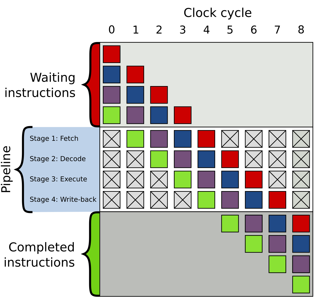
Ahmad Yasin's top-down method (ISPASS 2014) starts from how a core works. A core is built like an assembly line, called the pipeline: one end fetches and decodes instructions, the other end executes them, and on every cycle the line has a few slots where a new instruction could enter. Top-down sorts every one of those slots into four buckets:
| Bucket | The slot was… | Typical cause |
|---|---|---|
| Retiring | Used by an instruction that completed | Good; reduce instruction count to go faster |
| Bad speculation | Used by work thrown away | Branch mispredictions (chapter 01) |
| Frontend bound | Empty because instructions weren't fetched and decoded in time | Large code, instruction-cache misses |
| Backend bound | Empty because execution was waiting | Cache misses, long-latency operations |
On Intel, perf stat --topdown and toplev compute these from the counters. The method's value is that it tells you which of four very different fixes to try before you try any of them.
7.3When the counters aren't there
Many virtual machines don't pass the PMU through to the programs inside them, and containers running on those machines inherit the gap. The command below asks perf stat for the hardware counters and for two software ones, while running a small Python one-liner, in a container backed by a virtual machine.
perf stat -e cycles,instructions,cache-misses,task-clock,context-switches \
-- python3 -c "sum(range(10**6))" <not supported> cycles
<not supported> instructions
<not supported> cache-misses
22.47 msec task-clock # 0.992 CPUs utilized
0 context-switchesThe three hardware events print <not supported>, because the virtual machine doesn't pass the PMU through. The software events, task-clock and context-switches, are counted by the kernel and work fine. That's also why perf record still worked in section 5.4. By default it takes a sample each time the cycle counter has counted a set number of cycles, and with no cycle counter available it fell back to a kernel timer, which is the "timer ticks" of the scene in section 5.2.
What do you do then? Profile on hardware where the PMU is exposed (bare metal, or instance types that pass it through), or reason from timings instead: measure the same loop at several working-set sizes and watch for the steps chapter 02 shows at each cache level.
With the target found and the reason understood, we change the code. Then we need to find out whether the change helped.
08Benchmarks you can trust
In section 1 we checked our fix with a stopwatch, and the answer was 449 times faster, hard to argue with. Most real changes are worth 5% or 30%, and that's where measuring goes wrong. A benchmark is an experiment you build to answer one question, usually "is B faster than A?". It's the easiest tool in this chapter to get wrong, because a broken benchmark still prints a number.
8.1The compiler deletes what you don't use
The first trap is the compiler. A compiler translates source code into machine code, and at -O2 it rewrites the program to run faster, as long as the program's output stays the same. Two of its tricks matter here. Dead-code elimination removes work whose result is never used. Constant folding replaces a computation with its answer when the answer can be worked out at compile time. A close relative replaces a whole loop with a formula that gives the same result, so the loop never runs.
Here are three loops, each running N = 100 million iterations and timed in nanoseconds per iteration, compiled with -O2. Loop 1 adds up square roots and never uses the sum. Loop 2 adds the same square roots and prints the sum afterwards. Loop 3 adds up i * i with integers and prints the sum, which has a closed-form formula.
// 1: result never used
double s = 0;  for (int i = 0; i < N; i++) s += sqrt((double)i);
// 2: result printed afterwards
double s2 = 0; for (int i = 0; i < N; i++) s2 += sqrt((double)i);
// 3: result printed, but it has a closed form
uint64_t s3 = 0; for (uint64_t i = 0; i < N; i++) s3 += i * i;unused result: 0.000 ns/iter
used result: 0.585 ns/iter (sum=6.66667e+11)
closed form: 0.000 ns/iter (sum=662921401752298880)Two of the three loops cost nothing. The -O2 assembly contains exactly one loop: loop 1 was deleted because nothing reads s, and loop 3 was replaced by a formula for the sum of squares. Only loop 2 did real work, at about 0.585 ns per iteration, and repeated runs give the same numbers. With optimisation off (-O0) all three loops take between 0.5 and 0.9 ns per iteration, so the zeros come from the compiler and not the loops.
A benchmark that reports zero is easy to spot. The dangerous case is a benchmark where the compiler deletes part of the work and the number looks plausible.
?How do real harnesses prevent it?
By making the result escape somewhere the compiler can't see through. JMH (the Java benchmark harness) passes results to a Blackhole, Google Benchmark has DoNotOptimize, and Rust has std::hint::black_box. They also vary the inputs, so constant folding can't precompute the answer.
8.2The JIT hasn't finished yet
On a JVM, the code you time in the first second isn't the code you'll run in production. It starts in the interpreter, which executes it slowly one step at a time. OpenJDK's JVM has two JIT compilers. Once a method has run often enough to count as hot, the quick one, called C1, compiles it into reasonable machine code. If it stays hot, the slower and more thorough one, C2, compiles it again with heavy optimisation. A benchmark that stops its clock early measures the slow versions.
This loop hashes a 10,000-element array 200 times per batch, for twenty batches, in one JVM, repeated across seven runs:
| Batch | Fastest of 7 runs | Median of 7 runs |
|---|---|---|
| 1 | 6.2 ms | 7.2 ms |
| 2 | 1.7 ms | 4.7 ms |
| 10 | 1.8 ms | 2.3 ms |
| 20 | 1.7 ms | 1.8 ms |
| 20, interpreter only (-Xint) | 77 ms | 92 ms |
These are OpenJDK 21 numbers, taken on a busy shared host, so the medians are noisy (section 8.3 is about that). Even the fastest runs show the pattern: the first batch was roughly 3.6× slower than steady state, and interpreted code roughly 45× slower.
8.3Run-to-run noise
Even a program that never changes takes different times from one run to the next. The same binary from section 5.4, run eleven times back to back on a shared container, took between 2.8 and 5.8 seconds. Nothing changed between runs except what the other tenants, the other programs and customers sharing that hardware, were doing.
How does anyone benchmark on a shared machine? By controlling what they can and reporting the rest honestly. In the table, taskset pins a program to chosen cores, and the governor is the kernel setting that decides how fast the CPU clock runs:
| Source of noise | What it does | Control |
|---|---|---|
| Other tenants, other processes | Steals CPU, cache and memory bandwidth | Dedicated hosts; pin with taskset; interleave A and B runs |
| CPU frequency scaling and turbo | The same work takes different time | Fix the governor; or measure cycles, not seconds |
| Thermal throttling | Later runs slower than early ones | Interleave A and B, don't run all of A then all of B |
| Memory layout | Alignment changes cache and branch behaviour | Randomise layout (next section) |
| Timer resolution | Short operations round to zero | Time batches, not single calls |
For CPU-bound microbenchmarks, Chen and Revels argue for the minimum as the estimator, since noise only ever adds time. For anything a user waits on, report the distribution (p50, p99, max), because the noise is part of what the user experiences.
8.4Measurement bias
Noise is random and you can average it away. Some errors don't average away, because they're the same on every run. Mytkowicz, Diwan, Hauswirth and Sweeney's ASPLOS 2009 paper, Producing Wrong Data Without Doing Anything Obviously Wrong!, is the one to read before you trust a 5% result.
They changed things that shouldn't matter: the size of the UNIX environment (an unused environment variable) and the order object files were linked. Changing the environment size alone changed a program's run time "frequently by about 33% and once by almost 300%", because the environment sits above the stack and shifts every stack variable's alignment.
That matters for your A/B test because the bias can flip the conclusion. Across link orders, the measured speedup of -O3 over -O2 for perlbench (the Perl benchmark in the SPEC suite) ranged so widely that "we may think we have a 7% slowdown when in fact we have a 8% speedup". The username is stored in the environment, so your optimisation can win or lose depending on who ran the benchmark.
Their remedy is setup randomisation: run each variant under many environments and layouts and compare distributions, so no single lucky layout decides the result.
8.5Microbenchmarks versus the real thing
A microbenchmark times one small piece of code in isolation. A macrobenchmark, or load test, drives the whole service with realistic traffic. They answer different questions. Two abbreviations in the table: GC is garbage collection, the pauses a runtime takes to free memory, and L1 is the CPU's smallest, fastest cache.
| Microbenchmark | Macrobenchmark / load test | |
|---|---|---|
| Question | Is this function faster? | Does the service meet its latency target at this load? |
| Strength | Isolates one change; fast to iterate | Includes contention, GC, I/O, the network |
| Classic lie | Data fits in L1; branch predictor learned the pattern | Load generator hides stalls (coordinated omission) |
| Report | Minimum or median, with spread | Latency percentiles at a fixed offered rate |
A function that got 30% faster on a 4 KB input might well get slower on production inputs that don't fit in cache, so always finish with the macro test.
Load tests have their own traps. In coordinated omission, the load generator stops sending requests while the server is stalled, so the stall never shows up in the numbers. It's covered in chapter 16, and running load tests for capacity is in chapter 42.
Every profiler and benchmark in this chapter also costs something to run, and that cost decides which of them you can afford to leave on all the time.
09What measuring costs
Profiling takes something from the system it watches: CPU for the samples and disk for the files. Here are the numbers from the sections above, side by side.
Now put the overhead next to what a profile can find. Say a service uses 500 cores' worth of CPU. Turning on frame pointers costs 1% to 2% of that, and a profile then finds a function that owns 10% of the CPU and can be made twice as fast. Section 2.2 says that saves 5%.
| CPU the service uses (an example) | assumed | 500 cores |
| Cost of frame pointers, 1% to 2% | 500 × 0.01 to 500 × 0.02 | 5 to 10 cores |
| Fix a function owning 10%, twice as fast: a 5% saving | 500 × 0.05 | 25 cores |
| one profile-guided fix | pays for frame pointers 2.5× to 5× over | |
Always-on profiling is cheap enough to leave running only if the stack walk is cheap, which means frame pointers. DWARF unwinding gives nearly the same ancestry for about 66 times the data per sample, so disk space that holds a year of frame-pointer profiles holds less than a week of DWARF ones.
10Keeping it fast
A fix that works today can be undone by next month's release. Most performance problems are introduced one small release at a time, so the cheapest time to catch one is the day it lands.
10.1Benchmarks in CI
Run a small benchmark suite on every merge, on the same dedicated machine, and compare against a stored baseline. Flag a change only when the difference is larger than the run-to-run spread that machine shows.
?Why not a fixed threshold like 5%?
Because the noise floor differs per benchmark (section 8.3). A test whose runs spread by 8% will alarm constantly at a 5% threshold, and one that spreads by 0.5% will hide a 4% regression. Compare each benchmark against its own measured spread, with a statistical test such as Mann-Whitney U, which doesn't assume a normal distribution.
10.2Continuous profiling in production
Sampling at 99 Hz costs little enough to leave on. Continuous profilers (Google-Wide Profiling, Parca, Pyroscope, Datadog's and others) sample every host all the time and store the folded stacks. When a release regresses, you diff this week's fleet profile against last week's, which is the differential flame graph of section 6.4 applied to a whole fleet.
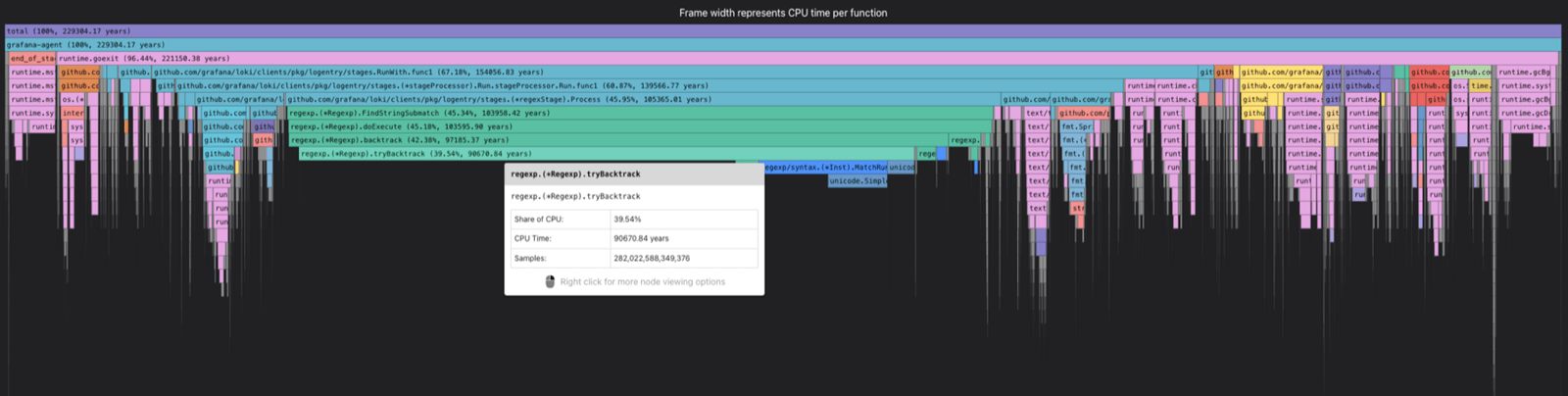
The frame-pointer argument from section 5.5 is what makes this practical. Without frame pointers, always-on profiling means DWARF unwinding on every host, and that section measured what DWARF does to data volume.
11Working through a slow service
11.1Commands, by the question they answer
Each question this chapter raised has a command that answers it on a running Linux machine.
# Which endpoint, and since when? (section 4.1)
# RED comes from your metrics system: request rate, error rate and p50/p99 duration per endpoint.

# Is a resource saturated? (sections 4.2 and 4.3)
dmesg -T | tail                  # errors first
vmstat 1                         # r above the CPU count means a queue for cores
cat /proc/pressure/cpu           # PSI: time stalled waiting for CPU
iostat -xz 1                     # %util, queue size and await for disks
nstat                            # retransmits, listen overflows

# Is the container being throttled? (section 4.4)
cat /sys/fs/cgroup/cpu.max /sys/fs/cgroup/cpu.stat

# Which code is using the CPU? (sections 5 and 6)
perf record -F 99 -g -- ./myprogram
perf script | ./stackcollapse-perf.pl | ./flamegraph.pl > flame.svg
perf record -F 99 --call-graph dwarf -- ./myprogram     # if frame pointers are missing

# Why is that code slow? (section 7)
perf stat -e cycles,instructions,cache-misses -- ./myprogram
stackcollapse-perf.pl and flamegraph.pl come from Gregg's FlameGraph repository. The first folds the output of perf script into the format of section 6.1, and the second draws the SVG.
11.2From complaint to fix
- Write down the goal and the number. "p99 of
/reportfrom 180 ms back under 100 ms at 2,000 req/s." (Section 2.) - RED on the service. Which endpoint, since when, correlated with which deploy or traffic change? (Section 4.1.)
- USE on the hosts and pools behind it. Errors first, then saturation. In containers, check throttling. (Sections 4.2 to 4.4.)
- On-CPU or off-CPU? Compare CPU time to wall time for slow requests. (Section 3.)
- Profile the right kind. CPU flame graph for on-CPU; off-CPU graph or lock and pool metrics for waiting. (Sections 5 and 6.)
- Form one hypothesis and test it with one change. A benchmark if it's a function, a load test if it's the service. (Section 8.)
- Confirm in production with the same RED metric you started from.
11.3Rules that hold up
- Measure before you change anything, and rank candidates by the share of time they own.
- Compare CPU time to wall time before you open a CPU profiler.
- Check saturation first on every resource, including pools, locks and container CPU quotas.
- Build with frame pointers so production profiles have ancestry.
- Attach conditions to every benchmark number: hardware, flags, input size, warm-up, repetitions and spread.
- Interleave A and B runs, and report distributions for anything a user waits on.
- Finish with a macro test at production input sizes before calling a change a win.
11.4What you trade for what
| You get | You pay | When the bill arrives |
|---|---|---|
| Profiles with ancestry (frame pointers) | 1% to 2% CPU, and a build flag in every service | As a small, permanent overhead |
| Exact timings from a tracing profiler | A program slowed enough that the timings change | As a profile that misleads you |
| Cheap always-on profiling (sampling) | Statistical answers: rare functions barely show up | When a rare, slow path is the problem |
| Reproducible benchmarks on a dedicated host | Hardware that mostly sits idle | As a CI bill |
| Fixed regression thresholds | False alarms on noisy tests, misses on quiet ones | As alert fatigue or a slow leak of speed |
11.5Symptom, cause, fix
| Symptom | Likely cause | Fix |
|---|---|---|
| Latency up, CPU flame graph unchanged | Time is off-CPU: locks, I/O, pools | Off-CPU profile; pool and lock metrics |
| Container slow, node CPU looks idle | CPU quota throttling | Check cpu.stat; raise or remove the limit; smooth bursts |
| Flame graph stacks one or two frames deep | No frame pointers | Rebuild with -fno-omit-frame-pointer, or --call-graph dwarf short-term |
Profile all [unknown] | Symbols unavailable: JIT, container path, stripped | async-profiler, perf maps, --symfs, debug packages |
| Benchmark says 0 ns, or implausibly fast | Dead-code elimination or constant folding | Blackhole / DoNotOptimize; varied inputs |
| JVM benchmark improves every run | JIT warm-up inside the measurement | JMH with warm-up iterations and forks |
| A/B result flips between machines or days | Noise or measurement bias | Interleave runs, randomise setup, report spread |
| Fast function, slow service | Microbenchmark didn't match production data or contention | Macro load test at production input sizes |
| Low IPC in a hot loop | Stalled on memory | Improve locality; see chapter 02 |
12Summary
- Measure before you change anything. The profile of the report put 99.8% of the time in one loop, and fixing that loop made it about 449 times faster.
- Name the goal first. Latency, throughput and efficiency pull in different directions, and "faster" has to mean one of them.
- Amdahl caps every optimisation. Doubling the speed of a 10% slice saves 5%, so rank work by share of time.
- Split on-CPU from off-CPU time. A CPU profiler can't see a thread that's waiting, and in the example request 195 of 200 ms were waiting.
- RED finds the service, USE finds the resource. Saturation is the column that predicts latency.
- Containers hide a saturation. In the example container, 41% of CPU periods were throttled while the node had idle cores.
- A sampling profiler is an interrupt plus a stack walk, and the walk follows frame pointers, a linked list the compiler may not have built.
- Without frame pointers the ancestry breaks. In the toy profile,
mainappeared in 2 of 2,649 samples instead of all of them. DWARF recovered 87% at 66× the data. - A flame graph's width is share of samples, and its x-axis isn't time. Read wide plateaus, check a hot leaf's callers, and diff two profiles to find a regression.
- Compilers and JITs rewrite benchmarks. Unused results are deleted, closed forms are folded, and cold JVM code ran 3.6× slower than warm.
- Shared machines and innocent setup changes bias results. Interleave runs, randomise setup, and report spread with every number.
13Build this
A profiling and benchmarking kit for one service.
- Rebuild a service you own with frame pointers, profile it under load with
perf record -F 99 -g, fold the stacks, and draw a flame graph. Then do it without frame pointers and compare the ancestry of its top three leaves. - Write a script that prints a USE pass for one host:
vmstat, PSI,iostat,nstat, and the cgroup'scpu.statthrottling ratio. - Take one hot function from the flame graph and benchmark it with a real harness (JMH, Google Benchmark,
criterion). Break it on purpose three ways, with an unused result, no warm-up and a cache-resident input, and record how far each moves the number. - Make a change, profile before and after, and produce a differential flame graph that shows it.
14Interview questions
beginnerWhat's the USE method, and how is it different from RED?›
USE checks every resource for utilisation, saturation and errors: CPUs, memory, disks, NICs, and software resources such as pools and locks. RED checks every service endpoint for rate, errors and duration. RED tells you which service is hurting users and since when, and USE tells you which resource it's waiting on. Saturation is usually the most telling column, because it measures the queue directly.
beginnerWhy sample at 99 Hz instead of 100 Hz?›
To avoid sampling in lockstep with periodic activity. Lots of software runs on 10 ms timers, and sampling at exactly 100 Hz could keep catching the same phase of that timer and skew the profile.
intermediateHow do you read a flame graph?›
Each box is a function in a stack, its width is the share of samples containing it, and its parent is its caller. The x-axis is sorted alphabetically so that identical stacks merge, which means left-to-right order says nothing about time. Look for wide boxes near the top with narrow children (functions doing work themselves), check the ancestry of hot leaves, and search for things like malloc or lock to total them across stacks.
intermediateYour flame graph shows stacks that are only one or two frames deep. Why?›
Probably missing frame pointers. The kernel's default stack walk follows saved frame-pointer and return-address pairs, and code built with -fomit-frame-pointer breaks the chain. In the toy profile of section 5.4, only 2 of 2,649 samples reached main without frame pointers, against all of them with. Fix it by rebuilding with -fno-omit-frame-pointer (Fedora 38 and Ubuntu 24.04 now do this by default), or use --call-graph dwarf at the cost of much bigger data: about 66× in that profile.
intermediateA service in Kubernetes has high p99 but the node's CPU is 40% idle. What do you check?›
CPU throttling from the container's CPU quota. Read nr_throttled against nr_periods in the cgroup's cpu.stat, or the cAdvisor throttling metric. Bursty work can use a pod's whole quota early in each 100 ms period and then wait, which adds latency while the node looks idle. Then check off-CPU time and pools, since a CPU profile won't show either.
deepYour microbenchmark says the new version is 20% faster. What would make you not believe it?›
Dead-code elimination or constant folding (is the result consumed, are inputs varied?). JIT warm-up inside the timed region. An input that fits in cache when production data doesn't. Noise, if the difference is within run-to-run spread. And measurement bias from layout, which Mytkowicz et al. showed can move results by tens of percent and flip a conclusion. I'd want interleaved runs, a real harness, the spread, and a macro test at production input sizes.
deepWhen is a CPU profile the wrong tool?›
When the time isn't on the CPU: locks, I/O, pool waits, throttling, scheduler delay. A blocked thread executes no instructions, so a sampling CPU profiler never sees it. Compare CPU time to wall time for slow requests. If they differ a lot, use off-CPU profiling (stacks at sched_switch, weighted by blocked time), lock contention stats and pool metrics instead.
deepWhat does top-down analysis tell you that a flame graph doesn't?›
The flame graph says where the hot code is, and top-down says why it's slow. It classifies each pipeline slot as retiring, bad speculation, frontend bound or backend bound. Backend bound with low IPC points at memory stalls and data layout, bad speculation at unpredictable branches, frontend bound at code size, and retiring-dominated code at doing fewer instructions. Each needs a different fix, and the counters say which to try first, if the PMU is exposed at all.
15Go deeper
Two boxes sit side by side in a flame graph. Did the left one run first?›
No. The x-axis is sorted alphabetically so identical stacks merge. It carries no time information.
Your benchmark reports 0.000 ns per iteration. What happened?›
The compiler removed the work, either because the result was never used or
because it computed a closed form. Consume the result through a barrier such
as Blackhole or DoNotOptimize, and vary the input.
perf stat prints <not supported> for cycles. Can you still profile?›
Yes, with software events: perf record falls back to a timer-based
cpu-clock or task-clock sample. Hardware counters such as IPC need a PMU
the VM exposes.
Where does off-CPU time come from in a flame graph?›
From stacks captured when a thread blocks, at the scheduler's switch point, weighted by how long it stayed off the CPU.
The method, the Linux checklist, and the reasoning for software resources. brendangregg.com/usemethod.html.
The paper describing flame graphs, their variants, and how to read them. Companion page with tools: flamegraphs.html.
The history of the 2004 default, the overhead numbers, and the alternatives. Blog post.
The user-space frame-pointer walker perf uses on arm64, quoted in 5.3. Source.
Environment size and link order bias SPEC results enough to flip conclusions. ACM DL.
The statistics behind Julia's BenchmarkTools, and the case for the minimum. arXiv:1608.04295.
The four-bucket pipeline breakdown behind VTune and toplev.
Paper.
Rate, errors and duration for every service, and how it relates to USE. Grafana blog.
16Related chapters
Why saturation turns into latency, lock convoys a CPU profile can't see, and coordinated omission in load tests. Chapter 16.
Load testing for capacity, sizing a fleet, and autoscalers. Chapter 42.
What a low IPC is usually waiting for, measured from L1 to DRAM. Chapter 02.
How off-CPU profilers and tracing tools attach to the scheduler. Chapter 48.