You keep user profiles in a database, and the table has outgrown one machine. It might be too big for the machine's disk, or too busy for its CPU. So you buy three machines and split the profiles among them. From now on, every read and write for "user 7" has to go to the one machine that holds user 7, and every client that talks to the database has to know which machine that is.
The obvious rule is to spread users out by number. User n goes to machine n mod 3, meaning the remainder after dividing n by 3. It balances perfectly, and it works until the day you buy a fourth machine. The rule becomes "n mod 4", and of the users numbered 0 to 11, nine now belong to a different machine than before. A cluster that has to copy three quarters of its data every time it grows is a cluster nobody wants to grow.
Deciding who owns what is called partitioning, and this chapter asks one question about it: when data is split across machines, how does each piece of it find its owner, and how much has to move when the cluster changes? We'll follow those twelve users from this first simple rule, through the designs real systems use to make growth cheap, to moving data while the system keeps serving traffic.
01Giving every key an owner
1.1Splitting the data
Let's give the pieces names. Each machine in the cluster is a node. Each record in the database is found by a key, such as the user number, and the record itself is the value. A slice of the data that lives together on one node is a partition. (Some systems call it a shard, and the two words mean the same thing here.)
If you've read the previous chapter, you'll know replication, which puts the same data on several nodes so that one can fail without losing anything. Partitioning does the opposite job: it puts different data on different nodes, so the total can be bigger than any one machine, and the work can be shared. Real systems do both. Each partition is replicated, so a node holds copies of several partitions, and each partition lives on several nodes. For the rest of this chapter we'll look at one copy of each partition, because the question we care about is where partitions go.
Every partitioning scheme has to answer two questions:
- Which partition does this key belong to?
- Which node holds that partition, and how does a client find out?
For the first few sections we'll treat them as one question, as our three-machine rule does: key to node, in one step. Section 2 pulls them apart, and that turns out to be the most useful idea in the chapter.
1.2Hash, then modulo
Our rule worked on user numbers, but real keys are often strings such as user:42, and you can't take a remainder of a string. So the first step is to turn the key into a number with a hash function. A hash function takes any key and returns a large number. The same key always gives the same number, and different keys give numbers that look random, so even keys like user:41 and user:42 land far apart. The second step is the remainder: hash(key) mod N, where N is the number of nodes. We'll write % for mod, as most programming languages do.
To follow the arithmetic in our heads, we'll pretend the hash of key n is just n itself. A real hash scrambles the numbers, and the later experiments use real ones, but nothing in this section depends on the scrambling.
The appeal of this rule is that it needs no lookup. Any client can compute the owner of any key from the key and N alone, without asking anyone. With three nodes, key 7 goes to node 1, because 7 % 3 = 1.
1.3What happens when a node joins
The rule balances the keys perfectly, and its weakness appears when N changes. Here's our twelve keys on three nodes, followed through the arrival of a fourth:
Look at the last frame and notice that the keys moved around among nodes that were already in the cluster. Key 4 left node 1 for node 0, and nothing about the new node asked for that. It moved only because the divisor changed, and a different divisor gives a different remainder for most keys.
A key stays put only when hash % 3 and hash % 4 happen to agree. For twelve keys that holds for 0, 1 and 2. In general, going from N to N+1 nodes leaves only one key in N+1 where it was, which means a fraction N/(N+1) of the keys moves. Try it before reading on.
1 million keys are spread across 10 nodes with hash(key) % 10. You add one node and switch to hash(key) % 11. Roughly what fraction of keys now belong to a different node?
Moving 91% of your data to add 10% capacity is a full reshuffle of the cluster. Every copy crosses the network, and while a key is in flight, requests for it can reach the wrong node. The best any scheme could do is move exactly the new node's fair share, 1/(N+1) of the keys, and move them all to the new node. The rest of this chapter is a search for schemes that get there.
The problem in hash % N is that the owner of a key depends on the number of nodes, which changes. That suggests the first fix: stop computing the owner from the node count at all.
02Fixed partitions and a map
2.1Splitting the two questions apart
Remember the two questions from section 1.1. Our rule answered both at once, so a change in the number of nodes changed every key's answer. Suppose we answer them separately. Pick a number of partitions when we create the system, and make it larger than the number of nodes we'll ever have. The first function maps a key to a partition, hash(key) % P, where P is that fixed number. The second is a small table that says which node holds each partition. We'll call it the partition map.
The first function never changes, because P never changes, so a key's partition is permanent. Adding a node changes only the table: we hand the new node a fair share of whole partitions from the others, copy exactly those partitions, and edit a few table rows.
?Why not just map each key straight to a node?
Because then any change to the set of nodes changes the mapping of keys, and changing the mapping of a key means moving its data. With a layer of partitions in between, adding a node means reassigning a few whole partitions: a small edit to a small map, followed by a bulk copy of exactly those partitions.
Here is the same growth as in section 1, with six partitions of two keys each. A key's partition is its number mod 6, and each node owns two partitions:
p1 (7 % 6 = 1) and key 1 is in p1 too. The partition map says node 1 owns p0 and p1.The new node got four keys where a perfectly fair share would be three, because partitions are lumps of two keys. With thousands of partitions the lumps are small, and the share gets as close to fair as you like. The cost is a bigger map, which is still tiny next to the data.
2.2Redis Cluster's 16,384 slots
Redis Cluster does exactly this. It calls its partitions hash slots, and there are always 16,384 of them. Here is how it picks a key's slot:
unsigned int keyHashSlot(char *key, int keylen) {
    int s, e; /* start-end indexes of { and } */

    for (s = 0; s < keylen; s++)
        if (key[s] == '{') break;

    /* No '{' ? Hash the whole key. This is the base case. */
    if (s == keylen) return crc16(key,keylen) & 0x3FFF;

    /* '{' found? Check if we have the corresponding '}'. */
    for (e = s+1; e < keylen; e++)
        if (key[e] == '}') break;

    /* No '}' or nothing between {} ? Hash the whole key. */
    if (e == keylen || e == s+1) return crc16(key,keylen) & 0x3FFF;

    /* If we are here there is both a { and a } on its right. Hash
     * what is in the middle between { and }. */
    return crc16(key+s+1,e-s-1) & 0x3FFF;
}
crc16 is the hash function. & 0x3FFF keeps the lowest 14 bits of the result, which is the same as % 16384 because 16,384 is a power of two. The slot count never changes, so a key's slot never changes. Only the slot-to-node map does.
The rest of the function handles curly braces. If a key contains {…}, only the text between the braces is hashed. This is a hash tag, and it lets you force related keys into one slot: {user:1000}:cart and {user:1000}:profile both hash only user:1000, so they live in the same slot on the same node, and commands that touch both keys work. Without the tag, the two keys would most likely sit in different slots, and a command that names both fails with a CROSSSLOT error.
Instagram did the same thing in Postgres. Their sharding post describes several thousand logical shards, each a Postgres schema, mapped to far fewer physical servers. Moving a logical shard moves a schema, and no key's shard ever changes.
2.3When the fixed number is too small
The partition count is the one number in this design you can't change later, and some systems make it small. Kafka, which stores streams of messages (chapter 23), splits each stream, called a topic, into partitions, and a message's key picks the partition. Its default partitioner is a plain modulo over the partition count:
    public static int partitionForKey(final byte[] serializedKey, final int numPartitions) {
        return Utils.toPositive(Utils.murmur2(serializedKey)) % numPartitions;
}?Why doesn't Kafka work like Redis Cluster here?
Kafka has the same two layers as Redis: a key picks a partition with the formula above, and a separate map says which server holds each partition. The difference is the size of the fixed number. A topic usually has tens of partitions, where Redis always has 16,384 slots, so a busy topic can outgrow its count. The only way out is to add partitions, which changes numPartitions in the formula, and that brings back the % N problem from section 1. Kafka's docs warn that "this partitioning will potentially be shuffled by adding partitions but Kafka will not attempt to automatically redistribute data in any way", and Kafka can't reduce the partition count at all. Existing messages stay where they are, new ones for the same key go to a different partition, and since Kafka only promises message order within one partition, the per-key order breaks across the change.
Fixed partitions work when you can name a count that is big enough, and when you can afford a map that every client consults. Sometimes you can't do either. A fleet of cache servers, for instance, has no central table to keep, and its nodes come and go all day. For that case we want a way to compute an owner that survives changes to the node set without a table.
03The hash ring
3.1Keys and nodes on one circle
The idea comes from Karger and colleagues' 1997 paper on consistent hashing, written for web caches. Hash the keys onto a circle of values, as a clock face has positions 0 to 11. Then hash the nodes onto the same circle, by hashing each node's name. Each node's spot on the circle is called its token. A key belongs to the first node you reach by walking clockwise from the key's position.
Take our twelve keys with the circle having twelve positions. Suppose hashing the names of three nodes places them at positions 2, 6 and 10:
Key 7 walks clockwise to position 10 and belongs to C. Key 11 wraps around the end of the circle and belongs to A. The stretch of keys between one token and the one before it, such as 7 to 10 for C, is an arc, and everything in an arc has the same owner. A real implementation keeps the tokens in a sorted array, and finds a key's owner by binary search, which halves the list at each step, so a lookup among T tokens takes about log T steps.
Now add a fourth node. Its name hashes to position 8, which cuts C's arc in two:
The property to remember is that when a node joins, every key that changes owner moves to that node. When a node leaves, its keys pass to the next node clockwise and nothing else moves. Compare that with the nine keys that shuffled among old nodes in section 1.
3.2Uneven arcs and virtual nodes
D got two keys where a fair share was three. That was luck, and with one token per node the luck can be much worse. Names hash to random positions, and random points on a circle leave some gaps several times longer than others. A node's share of the keys is the length of its arc, so some nodes get far more than their share.
The fix is to give each node many tokens, called virtual nodes. Each node's share is then the sum of many small arcs, and sums of many random lengths average out. When a node joins, it cuts many small pieces from many neighbours instead of one big piece from one, and when a node leaves, its load spreads across many nodes instead of landing on one.
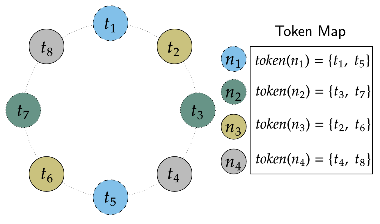
A simulation of 200,000 keys on 10 nodes growing to 11 shows the effect. With one token per node, the busiest node in the median run held 2.8 times its fair share. That is the node that fills its disk first, and it fills it nearly three times too early. With 256 tokens per node, the worst of nine layouts was only 16% over. Section 4.2 has the full table.
Balance is half the story. The other half is how many keys move when the cluster grows, and the next subsection lets you count them yourself.
3.3Trying it: count the moves
This script assigns 100,000 keys to five nodes two ways, adds a sixth node, and counts how many keys end up somewhere new. h hashes a string to a number with MD5. mod_owner is the rule from section 1. ring builds the circle, with 100 tokens per node placed by hashing node0#0, node0#1 and so on, and sorts them. ring_owner finds the first token after a key's hash using bisect, Python's binary search, and % len(points) wraps around from the end of the circle to the start.
import bisect, hashlib

def h(s): return int(hashlib.md5(s.encode()).hexdigest(), 16)

keys = [f"user:{i}" for i in range(100_000)]

def mod_owner(k, n): return h(k) % n

def ring(nodes, vnodes=100):
    pts = sorted((h(f"{n}#{v}"), n) for n in nodes for v in range(vnodes))
    return [p for p, _ in pts], [n for _, n in pts]

def ring_owner(k, r):
    points, owners = r
    return owners[bisect.bisect(points, h(k)) % len(points)]

old_nodes = [f"node{i}" for i in range(5)]
new_nodes = old_nodes + ["node5"]

moved_mod = sum(mod_owner(k, 5) != mod_owner(k, 6) for k in keys)
r_old, r_new = ring(old_nodes), ring(new_nodes)
moved_ring = sum(ring_owner(k, r_old) != ring_owner(k, r_new) for k in keys)

print("Add a 6th server to a cluster of 5 (100,000 keys)")
print(f"  hash(key) % N        : {moved_mod / len(keys):6.1%} of keys move")
print(f" consistent hashing : {moved_ring / len(keys):6.1%} of keys move (ideal: {1/6:.1%})")Add a 6th server to a cluster of 5 (100,000 keys)
hash(key) % N : 83.4% of keys move
consistent hashing : 16.8% of keys move (ideal: 16.7%)With hash % N, adding one node sent 83.4% of the keys to a different node. That matches the N/(N+1) rule from section 1.3, which gives 5/6 here. On the ring, only 16.8% moved, close to the ideal 1 in 6, which is exactly the share the new node has to receive.
Every moved key is data copied across the network, and while it moves, requests for it may hit the wrong node. A scheme that reshuffles 83% of the data whenever the cluster changes makes adding capacity a major event. A scheme that moves only the new node's share makes it routine.
3.4Tokens in a real database
Cassandra, a database built on a ring, calls the virtual nodes of a machine its tokens, and it used to give every node 256 of them. In version 4.0 it lowered the default num_tokens to 16. Fewer tokens make repair and streaming cheaper, because a node's data then lives in fewer separate pieces. Sixteen random tokens would give uneven shares, so Cassandra paired the change with a token allocation algorithm (allocate_tokens_for_local_replication_factor) that places a new node's tokens where they even out ownership, instead of at random.
The ring lets any client compute an owner from the list of nodes alone, but it still needs many tokens to balance well. Two newer schemes reach the ideal without a ring at all.
04Jump hash, rendezvous hashing and the rest
4.1Two ways to compute an owner
Jump consistent hash (Lamping and Veach, 2014) is a few lines of arithmetic that maps a 64-bit key to a bucket numbered from 0 to N−1. It needs no memory at all, moves the ideal 1/(N+1) of the keys on average when N grows by one, all of them to the new bucket, and balances almost perfectly. Its limit is that buckets are plain numbers, so you can only add or remove at the end. That is a good fit for a storage system whose shards are replicated and never disappear from the middle, and a poor fit for a cache fleet where any node can die.
Rendezvous hashing, also called highest-random-weight (Thaler and Ravishankar, 1998), works differently. For each key it scores every node with hash(key, node) and picks the node with the highest score. Remove any node, and only the keys it owned move, because the next-highest score takes over each one. The price is that every lookup computes one hash per node, which is fine for tens of nodes and slow for thousands.
4.2Side by side
Here are all the schemes on the same 200,000 keys, growing from 10 nodes to 11. The ideal is 9.1% of keys moved, since 1/11 is the new node's fair share, and a busiest-node figure of 1.00 would be perfect balance. The middle column divides the busiest node's key count by the average count. Where a node lands on a ring depends on its name, so the last column reruns the ring nine times with nine different sets of node names and reports the median run, with the worst run in brackets. The exact values depend on the node names and the hash function, so your own run will give different decimals, but the same pattern.
| Scheme | Keys moved (ideal 9.1%) | Busiest node ÷ mean | Busiest ÷ mean, median of 9 seeds (worst) |
|---|---|---|---|
| hash % N | 90.9% | 1.01 | — |
| Ring, 1 token per node | 13.7% | 2.31 | 2.77 (3.76) |
| Ring, 16 tokens per node | 11.4% | 1.36 | 1.31 (1.82) |
| Ring, 100 tokens per node | 9.4% | 1.14 | 1.19 (1.27) |
| Ring, 256 tokens per node | 9.1% | 1.07 | 1.11 (1.16) |
| Jump consistent hash | 9.1% | 1.01 | — |
| Rendezvous (HRW) | 9.2% | 1.01 | — |
Read the table from the top. hash % N balances perfectly and moves almost everything. A ring with one token per node moves roughly the right number of keys but leaves the busiest node with more than twice its share. Adding tokens fixes the balance gradually, and jump hash and rendezvous hashing balance almost perfectly with no tokens at all.
Each scheme has its own trade-offs, summarised below with the systems that use them. The "Weights?" column asks whether you can make one node take a bigger share, because its machine is bigger.
| Scheme | Lookup cost | Memory | Remove any node? | Weights? | Used by |
|---|---|---|---|---|---|
| Fixed slots | O(1) table lookup | Slot table | Yes, reassign its slots | By slot count | Redis Cluster, Instagram, Couchbase vBuckets |
| Ring + vnodes | O(log T) | T tokens | Yes | By token count | Cassandra, Riak, Dynamo |
| Jump hash | O(log N) arithmetic | None | Only the last | No | Storage shard selection |
| Rendezvous | O(N) hashes | Node list | Yes | Yes, with weighted scores | GitHub's GLB director (a variant) |
| Maglev | O(1) table lookup | Lookup table | Yes, with small disruption | Yes | Google's network load balancers |
Maglev hashing belongs to load balancing more than storage. It trades a little extra disruption on changes for a fast table lookup and near-perfect balance.
Every scheme in this section decides where a key lives by hashing it, and the property that makes hashing so good at spreading load also has a price. It scatters neighbouring keys. Keys 4, 5, 6 and 7 are neighbours in the key space, and they sit on three different nodes. That matters whenever a query asks for a stretch of keys.
05Keeping neighbours together: range partitioning
5.1Sorted keys, cut into ranges
Suppose the keys in our example are order numbers, and a query asks for orders 4 to 7. Reading a stretch of neighbouring keys in order is called a range scan, and databases do it constantly: all orders from one day, all messages in one conversation. With hashing, those four keys sit on three different nodes, so the query has to ask all three. If the neighbours lived together, one node could answer.
That's the idea of range partitioning. Sort the keys, cut the sorted order into contiguous ranges, and give each range to a node:
Google's Bigtable called these ranges tablets. HBase and TiKV call them regions, and CockroachDB calls them ranges.
5.2Splitting and finding ranges
Nobody chooses the cut points up front. A table starts as one range, and a range splits when it grows too big. In CockroachDB the default is to split at 512 MiB (range_max_bytes) and to merge adjacent ranges that fall below 128 MiB.
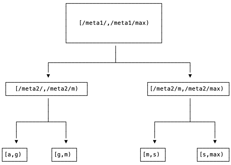
Finding a key's range is a lookup in a sorted index of range boundaries. CockroachDB stores that index in the key space itself, as two levels of meta ranges, and every node caches it. The diagram below follows one split. Real keys are usually strings, so it uses keys that start with letters instead of our numbers. [m, z) means every key from m up to, but not including, z:
m and z all land in one range, held (with its replicas) by node 2.Notice that this is the same two-step design as section 2. A split edits a small map, and the data only moves later, when the rebalancer decides to.
?Why split by load as well as size?
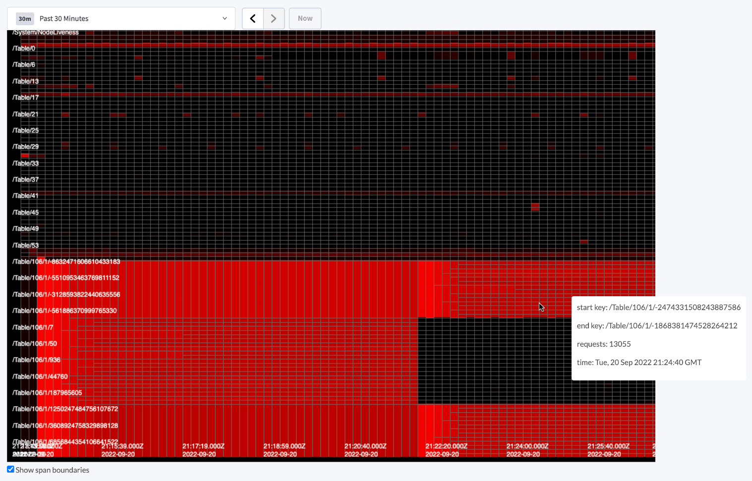
Because a small range can still be the busiest one in the cluster. CockroachDB's load-based splitting splits a range whose request rate crosses a threshold, choosing the split key from sampled requests so the two halves get similar load. Then the halves can live on different nodes.
5.3The hot-spot problem
Range partitioning has one weakness, and it appears when keys arrive in order. Suppose our keys are timestamps, and new keys 12, 13, 14 and so on keep arriving. They are all larger than every existing key, so every one of them lands in the last range, the one on N2. If the key is a timestamp, an auto-increment ID or anything that starts with one, every new write goes to the last range. Your cluster has fifty nodes and one of them takes all the inserts. A node that takes a disproportionate share of the traffic is called a hot spot.
?Why doesn't splitting fix a time-ordered hot spot?
Because the new half gets all the new writes too. Split [t0, now) into two and every insert still lands in the upper half. All that moves is the hot spot, to whichever node owns the newest range.
Every fix breaks the ordering on purpose. Two of them lead the key with a high-cardinality column, meaning one with many distinct values such as a user id, so that writes for different users fall in different places:
| Fix | How | What you lose |
|---|---|---|
| Prefix with a hash | Key = hash(user) % 16 + timestamp | Time-range scans become 16 scans |
| Lead with a high-cardinality column | Key = (user_id, timestamp) instead of (timestamp) | Global "latest events" queries |
| Random or hashed IDs | A random 128-bit ID (UUIDv4) instead of a sequence | Inserts no longer go to one end of the on-disk index (a B-tree), so they touch more pages; see the storage engines chapter |
| Hash-sharded index | CockroachDB's USING HASH does the prefixing for you | Ordered scans on that index |
5.4No scheme wins every row
We've now met two families, hashing and ranges, and each one gives up something the other keeps. Here are the goals a partitioning scheme has to balance, and what works against each:
| Goal | Why it matters | What works against it |
|---|---|---|
| Even data | No node runs out of disk first | Uneven key distribution, partitions of different sizes |
| Even load | No node saturates while others idle | Popular keys, time-ordered writes |
| Cheap scans | Range queries touch few partitions | Hashing, which scatters neighbouring keys |
| Cheap rebalancing | Adding a node moves little data | Schemes that tie key placement to node count |
| Local operations | Multi-key reads and transactions stay on one node | Any split of related keys |
Range partitioning keeps scans cheap and is prone to hot spots. Hash partitioning spreads load and makes range scans touch every partition. Even a perfect hash has a gap, though, because it spreads keys, and the load comes from requests.
06Hot keys and hot shards
6.1How skewed real traffic is
Hashing spreads keys evenly, and it does nothing about requests, because a single popular key always hashes to one place. When one user, product or hashtag gets a large share of traffic, the partition holding it is hot no matter how the keys were spread.
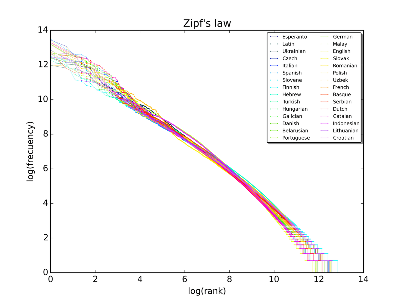
A common model for popularity is a Zipf distribution, where the k-th most popular key gets traffic proportional to 1/k. Simulating that over one million keys, hash-partitioned onto 10 nodes, gives these shares. The last row shows what salting does (section 6.2) when the 100 most popular keys are each split into 8 pieces:
| Share of all traffic | |
|---|---|
| Most popular single key | 6.9% |
| Fair share per node | 10.0% |
| Hottest node | 16.8% |
| Coolest node | 7.4% |
| Hottest node, top 100 keys each split 8 ways | 12.4% |
One key alone takes 6.9% of all traffic, most of a node's fair share. The hottest node ran at 1.68 times the average (the exact figure shifts with where the hash happens to put the popular keys), and adding nodes can't dilute a single key. At 100 nodes, that one key would still be 6.9% of traffic on one node, about seven times its fair share.
?Why can't the database just give the hot partition more room?
It can, up to the limit of one partition. DynamoDB, Amazon's hosted key-value database, states that every partition can serve at most 3,000 read units and 1,000 write units per second, where a unit is roughly one small read or write. Its adaptive capacity feature can isolate a hot item into a partition of its own, but then that item gets at most those 3,000 reads and 1,000 writes. Past that, only a change to the key design helps.
6.2What to do about a hot key
Since the cure can't be more nodes, every fix either takes load off the key's partition or splits the key itself:
| Technique | How it works | Cost |
|---|---|---|
| Cache the reads | Put a cache, or an in-process cache, in front of the hot key | Staleness; the cache is now the hot spot |
| Read from replicas | Spread reads over the partition's replicas | Replica lag; only helps reads |
| Split the key (salting) | Write to key#0 … key#7 at random; read all eight and combine | Every read fans out 8 ways |
| Write sharding with aggregation | Counters: increment a random sub-counter, sum on read or periodically | Reads are approximate or slower |
| Give it a dedicated partition | Detect hot keys and move them to their own node | Operational machinery to detect and move |
| Bounded-load hashing | Cap any server at c × average; overflow goes to the next server | Some requests land on a server without their cached data |
DynamoDB's own guide recommends write sharding with a random or calculated suffix, which is salting by another name.
Consistent hashing with bounded loads comes from Mirrokni, Thorup and Zadimoghaddam (2016), and HAProxy, a widely used load balancer, ships it as hash-balance-factor. From the HAProxy docs: "if <factor> is 150, then no server will be allowed to have a load more than 1.5 times the average", with 125 to 200 recommended.
So far every lookup has been by key. Real applications also ask for records by other columns, and partitioning by key does nothing for those.
07Queries that don't use the partition key
7.1Local indexes and global indexes
Partitioning by primary key makes lookups by primary key cheap, because the key says which partition to ask. Now suppose a user table is partitioned by user number, and someone asks for the user with a given email address. The user number isn't in the question, so the partitioning can't say where to look. The usual answer is an index, a lookup table from email to user number, and an index on anything other than the partition key is a secondary index. The question is where that index lives, and there are two answers:
| Local (per-partition) index | Global index | |
|---|---|---|
| Where it lives | Each partition indexes its own rows | The index is partitioned by the indexed value |
| Write cost | One partition, same transaction | A second partition, usually asynchronous |
| Read by indexed value | Ask every partition (scatter-gather) | Ask one index partition, then fetch rows |
| Consistency | Same as the base table | Often eventually consistent |
| Examples | Elasticsearch, Cassandra secondary indexes, DynamoDB local secondary indexes | DynamoDB global secondary indexes, CockroachDB and Spanner indexes |
"Eventually consistent" means a reader may briefly see the old state before the update arrives (chapter 28 covers what that costs you).
?Why is scatter-gather worse than it sounds?
Because a query that asks every partition is as slow as the slowest partition. With 100 partitions, a reply that is slow one time in a hundred turns up in about two queries out of three (1 − 0.99100, roughly 63%). The contention and tail latency chapter shows how fan-out amplifies the slowest few percent of replies, and it applies to every scatter-gather read.
DynamoDB shows the trade-off in its API: global secondary indexes can only be read with eventual consistency, because they're updated asynchronously from the base table.
7.2Keep things that change together together
Operations that touch several partitions need coordination: a distributed transaction, or a saga (a series of local steps with undo steps for failure), or an application that tolerates partial results. The distributed transactions chapter covers those. A cheaper fix is to avoid them by choosing a partition key that keeps related data together.
| Workload | Good partition key | Why |
|---|---|---|
| Multi-tenant SaaS | tenant_id | Almost every query is inside one tenant |
| Chat | conversation_id | Messages are read and written per conversation |
| Orders and their line items | customer_id, with items stored under it | An order and its items commit together |
| Time-series metrics | (series_id, time bucket) | Spreads writes across series, keeps one series' range scan local |
Redis hash tags (section 2.2), the vindexes of Vitess (a system that partitions MySQL, which we'll meet again in section 9) and the interleaved tables of Spanner (Google's distributed database) are all ways of saying "put these rows on the same shard".
Throughout the chapter we've assumed that a client can find out which node owns a partition. Where that knowledge lives is the next question.
08Routing: who holds the map
8.1Four places to keep the map
Once partitions can move, a client needs a current map from key to node, and the map is a piece of state like any other, with a home. There are four common places to keep it.
| Where the map lives | How a request finds its node | Examples |
|---|---|---|
| Smart client | Client caches the map, and servers redirect when it's stale | Redis Cluster (MOVED, ASK), Kafka clients, token-aware Cassandra drivers |
| Proxy tier | Clients talk to a proxy that routes | Vitess vtgate, MongoDB mongos, twemproxy, Envoy's Redis proxy |
| Any node forwards | Client talks to any node, which forwards or coordinates | Cassandra coordinators, CockroachDB gateways |
| Metadata service | An authoritative store holds the map; everyone watches it | ZooKeeper or etcd, Kafka's KRaft controller, CockroachDB meta ranges |
A client's cached copy can always be out of date, so every design has to say what happens then. In the smart-client row, the answer is a redirect: the node the client asked says "not mine, try that one", and the client refreshes its map. Section 9.2 shows Redis doing exactly that.
?Why does the map need consensus?
Because two nodes that both believe they own a partition will both accept writes for it, and nothing afterwards can merge those writes safely. The data itself may tolerate being a little stale, but ownership can't have two answers at once. So the map must be agreed on by a group of machines that follow a consensus protocol, and that's why it lives in etcd, ZooKeeper, a Raft group or (for Redis Cluster) behind an epoch number that only increases, so that every change of ownership carries a higher number and nodes ignore claims with an older one. The consensus chapter explains why those are safe, and the failure detection chapter covers what happens when a node wrongly believes it still owns something.
The map has to change whenever data moves, and in a live system data has to move while clients keep using it.
09Moving data without downtime
9.1The general recipe
Adding capacity means moving some partitions to new nodes while clients keep reading and writing them. Let's go back to our six partitions and watch one of them, p1 (keys 1 and 7), move from node 1 to node 4 while traffic continues. The naive way is to stop writes, copy, and restart, which makes the data unavailable for as long as the copy takes. Every system that does this online follows the same shape, with different names for the steps. This is that shape:
p1 holds keys 1 and 7 on node 1, and the routing map sends both reads and writes for p1 there. The goal is to move it to node 4 without stopping either.In a real system the change log is the database's own: MySQL's binlog, Postgres logical replication, or Kafka. The verify step needs a tool built for it. The last step is delayed because, once writes go to node 4, you keep a reverse stream running for a while, sending node 4's changes back to node 1, so that node 1 stays current and you can fail back to it.
Vitess, the MySQL partitioning system from section 7.2, follows this recipe. Its resharding guide maps onto those phases one-to-one: Reshard create copies and streams, VDiff verifies, SwitchTraffic --tablet-types=rdonly,replica moves reads, SwitchTraffic moves writes, ReverseTraffic exists for the way back, and complete cleans up.
?Why switch reads before writes?
Because a read switch is harmless to undo and a write switch isn't. Once writes land on the targets, the source is stale, and failing back needs the reverse stream. Moving reads first lets you find a bad routing rule, a missing index or a cold cache while going back is still free.
9.2Redis Cluster: moving one slot live
Redis Cluster moves data a slot at a time, and it does it without a pause at all, by letting clients be redirected mid-migration. The source is MIGRATING the slot and the target is IMPORTING it. The order of messages matters here, so this is the sequence for slot 1649 moving from node A to node B:
redis-cli --cluster reshard) marks slot 1649 as IMPORTING on B and MIGRATING on A. A still owns the slot.The decision between those replies is made in a dozen lines of getNodeByQuery():
    /* If we don't have all the keys and we are migrating the slot, send
     * an ASK redirection or TRYAGAIN. */
    if (migrating_slot && missing_keys) {
        /* If we have keys but we don't have all keys, we return TRYAGAIN */
        if (existing_keys) {
            if (error_code) *error_code = CLUSTER_REDIR_UNSTABLE;
            return NULL;
        } else {
            if (error_code) *error_code = CLUSTER_REDIR_ASK;
            return server.cluster->migrating_slots_to[slot];
        }
    }
If the command's keys are all missing from this node, the reply is ASK with the target's address. The middle case is a multi-key command whose keys are split between the two nodes. It gets TRYAGAIN, an error, for as long as the migration is in progress, because neither node can run the whole command.
Here's the whole thing on a two-node cluster. cluster keyslot asks which slot a key hashes to. cluster setslot 1649 importing $A and migrating $B mark the two ends of the migration, where $A and $B stand for the two nodes' ids (each node reports its own with cluster myid). migrate … keys moves a batch of keys, and cluster getkeysinslot supplies the list. M=<one of the migrated keys> is a placeholder for any key that the migrate call moved, and -c makes redis-cli follow redirects the way a smart client would.
redis-cli -p 7291 cluster keyslot '{user:1000}:cart'        # 200 keys live in this slot
redis-cli -p 7292 cluster setslot 1649 importing $A
redis-cli -p 7291 cluster setslot 1649 migrating $B
redis-cli -p 7291 migrate 127.0.0.1 7292 "" 0 5000 keys $(redis-cli -p 7291 cluster getkeysinslot 1649 100)

M=<one of the migrated keys>
redis-cli -p 7291 get "$M"                   # a moved key, asked at the source
redis-cli -p 7292 get "$M"                   # same key at the target, no ASKING
redis-cli -p 7291 get '{user:1000}:k1'       # a key that hasn't moved yet
redis-cli -p 7291 -c get "$M"                # -c follows redirects
# ... migrate the rest, then SETSLOT 1649 NODE $B on both nodes
redis-cli -p 7291 get '{user:1000}:k1'1649
ASK 1649 127.0.0.1:7292
MOVED 1649 127.0.0.1:7291
v
v
MOVED 1649 127.0.0.1:7292Read the output line by line, one per get or keyslot command. The first line is the slot, 1649. The moved key, asked at the source, gets ASK: node A owns the slot but no longer has that key. The same key asked at the target without ASKING gets MOVED back to A, because B doesn't officially own the slot yet. The key that hasn't moved is answered by A as usual (v), and -c follows the ASK and ASKING for us, so the fifth line is the value too. After SETSLOT NODE, A answers MOVED for everything in the slot, so the last line points at B.
9.3How fast to move
Moving data competes with serving traffic for disk, network and CPU on both sides. Every mature system throttles it: Cassandra's stream_throughput_outbound, CockroachDB's rebalance snapshot rate settings, Kafka's replication quotas for partition reassignment.
?Why not rebalance automatically the moment a node looks dead?
Because "looks dead" is a guess, and moving its data is expensive. If a node is merely slow and the cluster starts copying its partitions elsewhere, the copying loads the other nodes, which can make them look slow too. That's why Kubernetes, which runs containers across a fleet of machines, waits five minutes by default before moving work off a node it can't reach. It's also why Cassandra never moves data on its own when a node fails. It marks the node down, other nodes save the writes it misses (Cassandra calls these hints), and when the node returns it catches up from the hints and from repair, a background comparison of the replicas. That guess is the subject of the next chapter.
That leaves the practical side: on a running cluster, how do you tell whether any of the problems from this chapter is happening to you?
10Running a partitioned system
10.1What to watch
The commands below are grouped by the question they answer, with the section that raised it. Output depends on your cluster. One needs a word of setup: redis-cli --hotkeys only works when Redis's eviction policy, the rule it uses to choose keys to drop when memory is full, is an LFU (least frequently used) one, because that policy is what makes Redis count how often each key is read.
# Is one node carrying more than its share of keys? (sections 1 and 3)
redis-cli --cluster check HOST:PORT     # slots and keys per node, and any slots left mid-migration
nodetool status                         # Cassandra: the Owns and Load columns per node

# Is one key taking too much traffic? (section 6)
redis-cli --hotkeys                     # needs an LFU maxmemory-policy

# Who owns this key, and is a move in progress? (sections 2, 8 and 9)
redis-cli cluster keyslot KEY           # which slot a key hashes to
redis-cli cluster nodes                 # who owns which slots; look for migrating and importing
nodetool netstats                       # Cassandra: data streaming between nodes right now
Beyond commands, these are the quantities worth plotting:
- Per-partition size and request rate, not just per node. A node average hides one hot partition. Plot the busiest partition against the median.
- The skew ratio: busiest node ÷ mean, for disk and for requests. Above about 1.5, find out why before you add hardware.
- Top keys.
redis-cli --hotkeys(with the LFU policy above), DynamoDB's CloudWatch Contributor Insights, or sampled request logs. - Redirects and retries. A steady rate of
MOVED, stale-routing errors or Kafka'sNotLeaderOrFollowermeans clients hold a stale map. - Movement in progress. Bytes remaining in rebalancing and its throttle, so a slow migration is visible before it's a surprise.
10.2Rules that hold up
- Separate the key-to-partition function from the partition-to-node map, and never change the first (section 2).
- Pick a partition count that covers years of growth wherever the count is fixed at creation, as in Kafka and Elasticsearch (section 2.3).
- Never use
hash % Nwith N as the number of nodes when nodes come and go (section 1). - Give ring nodes many tokens, or use a token allocator (section 3).
- Choose a range-partitioned key by looking at write order. A leading timestamp makes one node take all the inserts (section 5.3).
- Salt only keys that measurement shows are hot (section 6.2).
- Verify before you switch when you move data online, and switch reads before writes (section 9.1).
10.3What you trade for what
| You get | You pay | When the bill arrives |
|---|---|---|
| Fixed partitions: cheap, explicit rebalancing | A count you can't change, and a map to store and keep correct | When the cluster outgrows the count |
| Hashing: even spread of keys | Range scans touch every partition | On the first query that scans |
| Ranges: cheap scans | Hot spots on ordered keys | At peak write load |
| A ring or jump hash: no central map | Uneven shares, or the limit of only adding at the end | As one node filling its disk first |
| Local secondary indexes: cheap writes | Scatter-gather reads | In the tail latency of every index query |
| Global secondary indexes: cheap reads | Slower, often eventually consistent writes | When a reader sees a stale index |
| Online resharding: no downtime | A copy, a log and a verification to run | As migration load on a busy cluster |
10.4Symptom, cause, fix
| Symptom | Likely cause | Fix |
|---|---|---|
| One node's disk fills first | Too few tokens per node, or uneven partition sizes | More vnodes or a token allocator; split big partitions |
| One node hot on writes; others idle | Time-ordered keys in a range-partitioned store | Hash-prefix the key, or lead with a high-cardinality column |
| One partition throttled; table far under capacity | A hot key | Cache, salt that key, or give it a dedicated partition |
| Adding a node triggers a huge data transfer | hash % N placement | Fixed partitions or consistent hashing |
| Per-key ordering broke after scaling a Kafka topic | Added partitions to a keyed topic | Create a new topic with more partitions and migrate consumers |
| Index queries slow, p99 worst | Scatter-gather over every partition | Global index, or a partition key that matches the query |
CROSSSLOT or TRYAGAIN errors in Redis | Multi-key command over keys in different slots, or mid-migration | Hash tags; retry TRYAGAIN with backoff |
("p99" is the latency that 99% of requests beat, so it measures the slowest few.)
11Summary
- Every scheme answers two questions: key to partition, and partition to node. Keeping them separate is what makes growth cheap, because the first never changes and the second is a small map.
hash % Nmoves almost everything. Going from 10 to 11 nodes moved 90.9% of keys in the simulation, and in our twelve-key example 9 of 12 moved, where the ideal is only the new node's share.- Many fixed partitions are the simplest fix. Redis's 16,384 slots and Instagram's logical shards never change a key's partition. Kafka and Elasticsearch fix the count at creation, so size them for years of growth.
- A ring moves keys only to the new node, and needs virtual nodes. With one token per node the busiest node held 2.8 times its share, and with 256 tokens, about 1.1 times.
- Range partitioning keeps scans cheap and invites hot spots. Time-ordered keys send every write to one node, and splitting doesn't help.
- Hashing spreads keys, not requests. One Zipf-popular key took 6.9% of all traffic, and no number of nodes dilutes it.
- Partitions have a ceiling. In DynamoDB it's 3,000 reads and 1,000 writes a second, even for a partition holding one isolated hot item.
- A secondary index is either local or global. Local indexes make reads scatter-gather over every partition, and global indexes make writes slower and often eventually consistent.
- The partition map needs consensus. Two nodes that both believe they own a partition will both accept writes.
- Online resharding is copy, stream, verify, switch reads, switch writes, clean up. Only the write switch pauses, and verifying is the step people skip.
- Redis Cluster redirects mid-migration with ASK, and afterwards with MOVED. A client that confuses them ping-pongs.
12Build this
A key-movement lab.
- Implement
% N, a ring with configurable virtual nodes, jump hash and rendezvous hashing over the same set of keys. Reproduce the table in section 4.2, then add node removal: remove node 3 of 10 and count moved keys. Jump hash can't do it directly; work out what you'd need to add. - Add weights: make one node twice as big and check that each scheme gives it twice the keys. Note which schemes make that easy.
- Start two Redis Cluster nodes and a writer that increments a counter under
{user:1}1,000 times a second. Migrate the slot by hand, as in section 9.2, and count errors the writer sees withredis-cli -cand with your usual client library.
13Interview questions
beginnerWhat's the difference between partitioning and replication?›
Replication keeps copies of the same data on several nodes, for durability, availability and read capacity. Partitioning splits the data so different nodes hold different subsets, for capacity and write throughput. Real systems combine them: each partition is replicated, so every node holds replicas of several partitions.
beginnerWhy is hash(key) % N a bad way to assign keys to nodes?›
Because changing N remaps almost every key. Going from 10 to 11 nodes changes the owner of about 10/11 of the keys, so adding 10% capacity moves roughly 91% of the data. Consistent hashing or a fixed number of partitions moves only the share the new node should own.
intermediateRange or hash partitioning for a table of events keyed by timestamp?›
Hash, or a range scheme with a hashed or high-cardinality prefix. Plain range partitioning on a timestamp sends every new write to the last range, so one node takes all inserts however many you add. If you need time-range scans, lead with something like (device_id, timestamp) or a hash bucket, and accept that a global time scan fans out.
intermediateWhat are virtual nodes and why do consistent-hash rings need them?›
Each physical node owns many positions (tokens) on the ring instead of one. With one token per node, arc lengths vary a lot: in the simulation the busiest of 10 nodes held about 2.8 times its share. Many tokens average out the arcs (about 1.1 times at 256), and when a node leaves, its load spreads across many nodes instead of landing on one neighbour.
intermediateOne celebrity's account overloads a shard. What are your options?›
Cache reads for that key; spread reads across replicas; split the key into N sub-keys (salting) and fan reads out; for counters, increment random sub-counters and sum them; or detect hot keys and give them a dedicated partition. Adding shards doesn't help, since one key always hashes to one place. Salt only the keys that are measurably hot.
deepIn Redis Cluster, what's the difference between MOVED and ASK?›
MOVED means the slot now belongs to another node permanently: update your slot map and send future requests there. ASK means the slot is mid-migration and this particular key has already moved: send this one request to the target, preceded by ASKING, and don't update the map. The target refuses requests for an IMPORTING slot without ASKING, answering MOVED back to the source.
deepWalk through resharding a live MySQL-backed service from 4 shards to 8.›
Create the 8 target shards. Copy a consistent snapshot of each source shard's rows into the targets by the new key ranges, recording the binlog position. Stream binlog changes from that position into the targets until lag is seconds. Verify with a row-level diff. Switch replica reads, then primary reads. Stop writes on the sources briefly, let the stream drain, flip the routing map to the targets and resume. Keep a reverse stream so you can fail back, then drop the old shards. Vitess automates exactly this as Reshard, VDiff, SwitchTraffic and complete.
deepWhy must the partition map be strongly consistent when the data isn't?›
Because two nodes that each think they own a partition will each accept writes, and nothing afterwards can merge them safely. The data may tolerate staleness; ownership can't. So the map lives in a consensus system (etcd, ZooKeeper, a Raft group, KRaft) or behind a monotonic epoch, and data nodes check the epoch on every request so an old owner's writes are rejected.
14Go deeper
What does & 0x3FFF do in Redis's keyHashSlot?›
It's modulo 16384, the fixed number of hash slots. It works as a bit mask because 16384 is a power of two.
Which keys move when a node joins a consistent-hash ring?›
Only keys on the arcs the new node's tokens cut off, and they all move to the new node. No key moves between two existing nodes.
Why can't jump consistent hash remove node 3 of 10 directly?›
Its buckets are the numbers 0 to N−1, and it can only grow or shrink N at the end. Removing a middle bucket needs an extra mapping layer on top.
A Redis MULTI touching two keys in a slot that's half migrated. What happens?›
TRYAGAIN, if the source holds some of the keys and not others. Retry after the migration step completes.
The original consistent-hashing paper, written for web caching. PDF
Jump consistent hash in five lines, with the proof that it's balanced and minimally disruptive. arXiv 1406.2294
Capping each server's load at c × average while staying consistent. arXiv 1608.01350
Slots, hash tags, MOVED and ASK, and the live resharding procedure, from the people who built it. redis.io
Online MySQL resharding, phase by phase, with the commands. vitess.io
Three partitioning strategies Amazon tried in production, ending with fixed equal-sized partitions assigned to nodes. PDF
15Related chapters
What each partition's replicas promise to readers, and quorum arithmetic. Chapter 28.
How the cluster decides a node is gone before it moves that node's partitions. Chapter 30.
The single-threaded server underneath each Redis Cluster node. Chapter 22.
What to do when an operation has to span partitions after all. Chapter 31.