You write one line of SQL:
SELECT sum(o.amount)
FROM orders o JOIN customers c ON o.customer_id = c.id
WHERE c.country = 'country_7';
It asks for the total of every order placed by customers in one country. Notice what the query leaves out. It says what result you want, and nothing about how to get it: which table to read first, whether to read every row or look rows up directly, how to match each order with its customer.
Someone has to decide those things, and the decisions matter more than you'd expect. Orders could be found by reading all five million of them, or by jumping straight to the few that belong to the customers we care about. The two tables could be matched in three quite different ways. Depending on what's chosen, the same query can finish in a few milliseconds or take half a minute. And the choice has to be made before the database has read a single row of the data, so it's made from a summary the database keeps about its tables.
Making the choice is the job of the planner. What it produces is a plan, a recipe of steps for getting the answer, and a second part, the executor, follows the recipe. This chapter follows the query above from text to result and keeps asking one question: how does the planner choose, and what is it looking at when it chooses badly? We'll start by asking a database to show us a plan.
01Ask the database for its plan
1.1One table, one lookup
Let's begin with the smallest case, one table and no join. The script below builds a table of 300,000 users, then looks up users by email address 200 times and reports the average time for one lookup. Next it puts EXPLAIN QUERY PLAN in front of the query. That is how you ask SQLite, the small database library that ships with Python, "how would you answer this?", and it prints the plan without running the query. Then the script adds an index on the email column and does everything again.
An index is a second, sorted copy of one column, where every entry also records which row it came from. It works like the index at the back of a book: instead of reading every page to find a word, you look the word up in the sorted list and go straight to the page. Save the script as plan.py.
The script times a lookup by email on 300,000 rows, adds an index on email, and times the same query again. How much faster is the second lookup?
import sqlite3, time

db = sqlite3.connect(":memory:")
db.execute("CREATE TABLE users (id INTEGER PRIMARY KEY, email TEXT, city TEXT)")
db.executemany("INSERT INTO users VALUES (?, ?, ?)",
               ((i, f"user{i}@example.com", f"city{i % 500}") for i in range(300_000)))
q = "SELECT id FROM users WHERE email = ?"

def timed():
    t = time.perf_counter()
    for i in range(200): db.execute(q, (f"user{i * 1500}@example.com",)).fetchall()
    return (time.perf_counter() - t) / 200 * 1000

print("plan :", db.execute("EXPLAIN QUERY PLAN " + q, ("x",)).fetchall()[0][3])
print(f"time : {timed():8.3f} ms per lookup\n")
db.execute("CREATE INDEX users_email ON users(email)")
print("plan :", db.execute("EXPLAIN QUERY PLAN " + q, ("x",)).fetchall()[0][3])
print(f"time : {timed():8.3f} ms per lookup")plan : SCAN users
time : 5.572 ms per lookup
plan : SEARCH users USING COVERING INDEX users_email (email=?)
time : 0.001 ms per lookupThe query text never changed, but the plan did. Before the index, the plan is SCAN users: the database reads every row of the table and tests each one, and a lookup takes about 5.6 ms. After it, the plan is SEARCH users USING COVERING INDEX users_email (email=?). SEARCH means the database jumps through the index using the condition email=? instead of reading everything, and COVERING means the index entry already holds everything the query asked for (the row's id), so the table itself isn't touched. A lookup now takes about a thousandth of a millisecond. A thousand lookups would spend 5.6 seconds on scans and about a millisecond on searches.
1.2What a plan is
A plan is the sequence of steps the database chose to produce your result. Reading it tells you which strategy was picked, and so whether the choice was a good one. It's a bit like a library. To find one book you can walk every aisle and read every spine, or you can look it up in the card catalog, which sends you to the right shelf. A good librarian doesn't do either by habit. They glance at how many books there are and how specific your request is, and then choose.
In the script above the planner had no real choice the first time, because there was no index, and it took the only road available. The second time it had two, and it took the faster one. In general the choices are many, and the planner can't try them all, because trying a plan means running it. It also can't look at the data first, because reading the data is most of the work. So it relies on statistics, summary figures the database keeps about each table: how many rows it has, how many distinct values each column holds, which values are most common. When those figures are wrong, the planner can pick the aisle walk over the catalog, and a query that took 5 ms takes 30 seconds. Section 7 is about how that happens.
SQLite printed one line of plan because the query touched one table. Our orders-and-customers query has two tables and a join, and its plan has several steps that don't run in a straight line. To read one, we first need to know how a query turns into a plan at all.
02From SQL to a running plan
2.1Two tables, one tiny and one real
Our query joins two tables. customers has one row per customer, with an id and the country the customer lives in. orders has one row per order, with an id, the customer_id of whoever placed it, and an amount. To follow what happens to the rows, we'll use a toy version of the data small enough to draw. It has four customers and eight orders:
customers: id | country |
|---|---|
| 1 | country_2 |
| 2 | country_7 |
| 3 | country_5 |
| 4 | country_7 |
orders: id | customer_id | amount |
|---|---|---|
| o1 | 2 | $20 |
| o2 | 4 | $10 |
| o3 | 1 | $15 |
| o4 | 3 | $40 |
| o5 | 2 | $5 |
| o6 | 1 | $25 |
| o7 | 4 | $30 |
| o8 | 3 | $15 |
Customers 2 and 4 are in country_7, so the answer to our query on the toy data is the sum of their orders: o1, o2, o5 and o7, which is $20 + $10 + $5 + $30 = $65. The timings later in the chapter come from a real database with the same two tables at a realistic size, which section 2.3 describes.
2.2Five stages
Every relational database sends a query through the same stages. The names differ between systems, but the jobs are the same. We'll use the names from PostgreSQL (usually just called Postgres), a widely used open-source database server, because its source code is public and we'll read some of it later. The parser reads the text and checks it follows SQL's grammar. The analyzer looks up every name in the catalog, the database's own record of which tables and columns exist and what types they have. The rewriter replaces views (saved, named queries) with the queries that define them. The planner, which we've met, picks a plan. The executor runs it. Here's our query going through all five:
orders exists.Planning is usually quick. For a simple query it takes roughly a millisecond or less, and that cost is the reason section 9 looks at plans that get reused.
2.3A plan is a tree of operators
What the planner hands over is a tree, and EXPLAIN prints it. Put EXPLAIN in front of any query in Postgres and it prints the plan it kept, without running the query.
To see a realistic plan we need realistic tables, so here is the real database promised in section 2.1. Postgres stores each table as a sequence of fixed-size pages, 8 KB each, and every read from a table fetches whole pages. In the test database, customers has 100,000 rows (736 pages), and orders has 5 million (41,667 pages, 326 MB) with indexes on customer_id, created_at, status and a random integer column r. Unless noted, queries ran on a single CPU core, with parallelism (splitting one query across several cores) and JIT (just-in-time compilation, which section 3 explains) both turned off, and all the data was already in memory. Most of the numbers in the rest of the chapter come from this database.
Here's the plan for our query on those tables:
 Aggregate  (cost=107056.82..107056.83 rows=1 width=32)
   ->  Hash Join  (cost=2011.25..106804.31 rows=101001 width=6)
         Hash Cond: (o.customer_id = c.id)
         ->  Seq Scan on orders o  (cost=0.00..91667.40 rows=5000040 width=10)
         ->  Hash  (cost=1986.00..1986.00 rows=2020 width=4)
               ->  Seq Scan on customers c  (cost=0.00..1986.00 rows=2020 width=4)
                     Filter: (country = 'country_7'::text)
Each line is one operator, also called a plan node, and a node's children are indented under it. Read the tree from the bottom. Seq Scan on customers reads every page of the customers table in order and keeps the rows whose country is country_7. Those rows go into a Hash, which is a lookup table the next node will use. Seq Scan on orders reads every order. Hash Join matches each order against the lookup table by customer_id, which is the join our SQL asked for. Aggregate at the top adds up the amounts of whatever reaches it. The numbers after each node are the planner's predictions, and they're what the planner used to make its choices:
| Field | Meaning |
|---|---|
cost=A..B | Estimated cost before the first row (A) and for all rows (B), in the planner's own units (section 6 defines them) |
rows | Estimated rows this node will return |
width | Estimated average row width in bytes |
?Why estimates and not facts?
Because the plan has to be chosen before anything runs. The planner can't know how many customers are in country_7 without reading the table, so it guesses from statistics gathered by ANALYZE, the command that samples a table and records its summary figures. Everything in this chapter follows from that: the choices are only as good as the guesses.
So a plan is a tree of nodes, and a tree on its own doesn't move any rows. Something has to carry rows from the leaves up to the root, and the way it does so decides how much CPU each row costs.
03How operators run
3.1The Volcano model: one row at a time
The simplest way to run a tree is to give every node one job: when asked for a row, return one. Each node has a single main operation, "give me your next row", usually called next(). A node that needs rows calls next() on its children as often as it needs to, does its own work on what comes back, and returns one row to whoever called it. Nothing is stored between nodes. Rows are pulled upward one at a time, on demand.
Goetz Graefe described this design in the Volcano paper (1994), so it's called the Volcano model, or the iterator model. Almost every row store, a database that keeps all the columns of one row together on disk, runs plans this way. Postgres, MySQL and SQL Server do. In Postgres the next() operation is a function called ExecProcNode, and every node carries a pointer to its own version of it:
static inline TupleTableSlot *
ExecProcNode(PlanState *node)
{
	if (node->chgParam != NULL) /* something changed? */
		ExecReScan(node);		/* let ReScan handle this */

	return node->ExecProcNode(node);
}
Everything happens on the last line, which calls whichever function this particular node uses: one for a table scan, another for a filter, another for a join. The first two lines restart the node from the beginning if a parameter it depends on has changed, which we'll need when we get to nested loops. Here is what pulling looks like on the customers half of our query. We'll count the customers in country_7, which is a scan under a filter under an aggregate (a node that counts or sums the rows it receives):
next() on the node below it.Notice that rows moved one at a time, and no node ever collected a batch of rows before passing them on.
?Why has this design lasted thirty years?
Because every node speaks the same next() language, any node can sit under any other, so a planner can assemble plans from a small kit of parts. And because rows are pulled on demand, the top of the tree controls how much work happens below it. A LIMIT 10 at the top stops calling next() after ten rows, and nothing below it does any more work.
Our plan has one more node worth reading: a join. Here is a whole join algorithm written against next(). A nested loop pulls one row from its outer input, restarts the inner input, and pulls inner rows until they run out. It's the first of three join algorithms, and section 5 explains when it's the right one. For now, look at how little the loop needs:
	for (;;)
	{
		if (node->nl_NeedNewOuter)
		{
			outerTupleSlot = ExecProcNode(outerPlan);
			if (TupIsNull(outerTupleSlot))
				return NULL;                    /* join is complete */
			/* ... pass outer values to the inner side as parameters ... */
			ExecReScan(innerPlan);
		}

		innerTupleSlot = ExecProcNode(innerPlan);
		if (TupIsNull(innerTupleSlot))
		{
			node->nl_NeedNewOuter = true;
			continue;
		}

		if (ExecQual(joinqual, econtext))
			/* ... project and return one joined row ... */
	}
Both inputs are asked for rows with the same ExecProcNode call. When the outer input runs out, the join is complete (return NULL). When the inner input runs out, the loop sets nl_NeedNewOuter and goes back to fetch the next outer row, restarting the inner side with ExecReScan, which is the restart the first function checked for.
3.2What one row at a time costs
This design charges per row. Each next() is an indirect call through a function pointer. Each expression, such as a % 7 = 3, is interpreted by walking a small tree of its own. Every column has to be pulled out of the row's stored format one at a time. None of that is the arithmetic you asked for.
Boncz, Zukowski and Nes measured how much of the time goes elsewhere in MonetDB/X100 (CIDR 2005). They profiled query 1 of TPC-H, a standard benchmark whose queries summarise large tables, on MySQL. The five operations doing the real work of the query "correspond to only 10% of total execution time". A single addition cost 38 instructions. Everything else went to hash-table work for the aggregate and to functions that "navigate through MySQL's record representation and copy data in and out of it".
3.3Vectorized and compiled execution
Two designs remove that overhead. A vectorized engine makes next() return a batch of roughly a thousand values for one column at a time instead of one row. Each operator then runs a tight loop over an array, so the per-row overhead is paid once per batch. A simple loop over an array is also what compilers optimise best: they can turn it into SIMD instructions, which apply one instruction to several values at once (chapter 01). A compiled engine goes further. For each stretch of the plan where rows flow from operator to operator without waiting for a whole input to be collected (called a pipeline), it generates machine code at run time, so a row can stay in the CPU's registers, its handful of fastest storage slots, from one operator to the next.
| Model | Idea | Systems | Strength |
|---|---|---|---|
| Volcano | One row per next() call, interpreted expressions | Postgres, MySQL, SQL Server row mode, SQLite (a bytecode VM with the same row-at-a-time shape) | Simple, composable, low memory |
| Vectorized | next() returns a batch (roughly a thousand values per column); each operator is a tight loop over arrays | MonetDB/X100 → Vectorwise, DuckDB, ClickHouse, Velox, SQL Server batch mode | Per-row overhead paid once per batch; loops the compiler can unroll and turn into SIMD |
| Compiled | Generate machine code for each query pipeline, keeping rows in registers between operators | HyPer, Umbra, Spark's whole-stage codegen | Fewest instructions per row |
Neumann's VLDB 2011 paper introduced the compiled approach using LLVM, a compiler toolkit, with code that "frequently rivals the performance of hand-written C++ code". When Kersten and colleagues built both in one system (VLDB 2018), they found "both are efficient": vectorization "is better at hiding cache miss latency", while compilation "requires fewer CPU instructions".
Postgres has a small piece of the compiled idea. Since version 11 it can compile expressions and the unpacking of rows with LLVM at run time (JIT), for queries whose estimated cost passes jit_above_cost, which is 100,000 by default.
3.4The same query, three engines
Here's the difference in practice. This test uses its own table, t5, with 5 million rows of an integer a and a double b, loaded from one CSV file into each engine. One engine needs a word of introduction. DuckDB is a column store: instead of keeping each row's columns together, as Postgres and SQLite do, it keeps each column in its own contiguous block. The query is select sum(b), count(*) from t5 where a % 7 = 3, and the times are the median of five warm runs, meaning the data was already in memory from an earlier run:
| Engine | Execution model | Time | ns per row |
|---|---|---|---|
| Postgres 16, 1 core, JIT off | Volcano, row store | 145 ms | 29 |
| Postgres 16, 1 core, JIT on | Volcano + compiled expressions | 130 ms | 26 |
| SQLite 3.45 | Bytecode VM, row store | 111 ms | 22 |
| Postgres 16, 4 parallel workers | Volcano, parallel | 86 ms | 17 |
| DuckDB 1.5.5, 1 thread | Vectorized, column store | 8 ms | 1.6 |
| DuckDB 1.5.5, 4 threads | Vectorized, column store | 3 ms | 0.6 |
DuckDB on one thread was 18 times faster than Postgres on one core. That probably isn't all execution model. Because DuckDB is a column store, it touches only the two columns the query needs. Postgres reads all 27,028 pages of the table and steps over the 23-byte header it stores with every one of the 5 million rows. Both effects point the same way, and that's why analytical engines combine columnar storage with vectorized execution.
Every engine in the table pays something per row it reads, and the fastest still pays 0.6 ns. Their biggest possible saving is to not read the rows at all. So the first decision in a plan is how to read each table.
04Reading one table
4.1Four ways to read a table
The 8 KB pages from section 2.3 hold a table's rows in no particular order, mostly the order they were inserted. Postgres calls this pile of pages the heap. A row's address in the heap is a page number plus its position inside the page. Postgres indexes are B+trees, sorted trees whose entries each hold a key and the address of the row it came from (chapter 18 builds one). The way a plan fetches rows from one table is called its access path. Postgres has four main ones, and each is a different answer to "find the orders of customers 2 and 4":
| Access path | How it works | Best when |
|---|---|---|
| Seq Scan | Read every page in order, test each row | A large fraction of rows match, or the table is small |
| Index Scan | Walk the B+tree for matching keys, fetch each row from the heap by its address (TID, a page number and position) | Few rows match, or rows are needed in index order |
| Index Only Scan | Answer from the index alone; check the visibility map instead of the heap | All needed columns are in the index and the table is mostly vacuumed |
| Bitmap Heap Scan | Collect matching addresses from one or more indexes into a bitmap, sort by page, then read each heap page once | A moderate fraction matches, or several indexes are combined with AND/OR |
The visibility map in the third row is a small per-page note that says "every row on this page is visible to everyone". Postgres keeps old versions of rows around (chapter 19), so an index entry alone can't say whether you may see its row, and the heap has to be checked. A page the map marks as all-visible lets the check be skipped, and VACUUM, the cleanup job, is what keeps the map current.
?Why would reading fewer rows ever be slower?
Because an index scan pays per row, and a sequential scan pays per page. An index scan on an unordered column jumps to a different heap page for almost every row, so fetching 5% of the rows can mean touching most of the pages, one at a time and out of order. A sequential scan reads all of them, but in order and with no index work at all.
4.2Index scan against bitmap scan
Let's watch the difference on the toy tables. Suppose orders has an index on customer_id and lives on four heap pages, two orders each: o1 and o2 on page 0, o3 and o4 on page 1, o5 and o6 on page 2, o7 and o8 on page 3. We want the orders of customers 2 and 4. An index scan follows the index entries one by one. A bitmap scan reads all the entries first and only then touches the heap.
With four orders the difference is one visit. On a table of five million rows, it's the difference between visiting each of 41,667 pages once and visiting pages in random order, again and again. A visit is a trip to a page even when the page is already in memory, because the database has to find it, check it and locate the row, and it's a trip to the disk when the page isn't in memory. Each visit costs time, and that makes the cost of an index scan grow with the number of matching rows, while a sequential scan pays one flat price for all the pages whatever matches.
So as more rows match, there must be a point, the crossover, where the index scan stops being the faster of the two. To find it on the real orders table, we can use two of its columns. r is a random integer, so matching rows are scattered across the table, as in the toy. id matches the physical order, since rows were inserted in id order. Each plan was forced with the enable_* settings (enable_seqscan and its siblings, which tell the planner to avoid one kind of plan, for experiments only). Before looking at the results, make a guess.
A query sums one column over rows where r < N, on a 5M-row table with r uniformly random. Everything is in memory. Forcing a plain Index Scan, at roughly what fraction of matching rows does it become slower than a Seq Scan?
The full results, each the median of five warm runs:
| Rows matching | Seq Scan | Index Scan (r, random) | Bitmap (r) | Index Scan (id, ordered) | Planner's choice for r |
|---|---|---|---|---|---|
| 0.01% | 162 ms | 0.2 ms | 0.2 ms | 0.1 ms | Bitmap |
| 0.1% | 160 ms | 1.1 ms | 1.8 ms | 0.4 ms | Bitmap |
| 1% | 164 ms | 57 ms | 57 ms | 3.1 ms | Bitmap |
| 5% | 169 ms | 270 ms | 96 ms | 16 ms | Bitmap |
| 20% | 183 ms | 1,224 ms | 157 ms | 71 ms | Bitmap |
| 50% | 221 ms | 2,969 ms | 270 ms | 194 ms | Seq Scan |
Three things stand out. A bitmap scan stays close to the better of the other two across the whole range, which is why Postgres picks it so often in the middle. The planner's choice for r was the fastest option, or tied with it, at every row except 0.1%, where it was under a millisecond behind. And on the ordered id column, the plain index scan beat the sequential scan even at 50%. That last result needs an explanation.
4.3Correlation: why order on disk matters
id behaves differently because of correlation: how closely the physical row order follows the column's sort order. ANALYZE measures it for each column, and the planner uses it to price index scans:
   attname   | correlation
-------------+--------------
 id          |            1
 customer_id |  0.002412658
 r           | -0.004186762
With correlation 1, consecutive index entries point at the same heap page, so an index scan over 50% of the rows reads about half the pages in order, which is almost what a sequential scan does and with fewer rows to test. With correlation near 0, every entry is a random page, like the toy's 0, 2, 0, 3. Time-ordered columns (an id from a sequence, created_at on an append-only table) are naturally correlated. Foreign keys such as customer_id, and hashes, aren't. CLUSTER rewrites a table in index order once, and the order isn't maintained as new rows arrive.
4.4Choosing which indexes to build
?What makes a good index for a query?
An index can cover several columns, sorted by the first, then by the second within each value of the first, like a phone book sorted by surname and then first name. This is a composite index. A good composite index starts with the columns the query compares with =, followed by at most one column it compares with a range (>, BETWEEN), so all the matching keys sit next to each other in the tree. After that, the aim is to avoid visiting the heap at all.
| Rule | Example | Why |
|---|---|---|
| Equality columns first, then one range column | (customer_id, created_at) for WHERE customer_id = $1 AND created_at > $2 | Matching entries are contiguous; with the range first, the equality can't narrow the scan |
| Cover the query to get an index-only scan | (customer_id) INCLUDE (amount) | No heap visit per row, if the visibility map is current |
| Index the rare value, not the column | CREATE INDEX ON orders (created_at) WHERE status = 'pending' | 0.1% of rows are pending; a partial index, which holds only the rows matching its WHERE, is 1,000 times smaller than a full one |
| Match the sort you need | (customer_id, created_at DESC) for ORDER BY created_at DESC LIMIT 20 per customer | The index delivers rows in order, so LIMIT stops after 20 |
| Don't index what's always scanned anyway | A status column where 99.9% of rows are done | The planner won't use it for done, and every write still pays to maintain it |
Now we can read each table. Our query still has two of them, and its answer needs rows from both matched up. How the matching is done has a bigger effect on the running time than anything in this section.
05Matching rows from two tables
Every join in every relational engine is done with one of three algorithms, or a variant of one. They differ in what they need from their inputs and in how their cost grows with the size of the tables. On our toy tables, each one has to pair customers 2 and 4 with o1, o2, o5 and o7. They go about it very differently.
5.1Nested loop
The most direct join is the one the source code above performs. For each row of one input (the outer side), look through the other input (the inner side) for rows that match. Take customer 2, scan all eight orders, and find o1 and o5. Take customer 4, scan all eight again, and find o2 and o7. With no index that costs O(N × M), the product of the two sizes. On the real tables, the roughly 2,000 customers in country_7 times 5 million orders is ten billion comparisons, so it's only sensible when one side is tiny.
The picture changes if the inner table has an index on the join column. Then each probe is a lookup in a B+tree instead of a scan, and customer 2's orders are found without looking at the other six. This index nested loop is the best join there is when the outer side is small. It's also the only algorithm that works for any join condition, including inequalities like a.ts BETWEEN b.start AND b.end.
5.2Hash join
For an equality join over larger inputs there's a cheaper way, and it starts from a data structure. A hash table finds a row by its key in one step: a function turns the key into a bucket number, and every row with that key is stored in that bucket. A hash join builds a hash table from the smaller input, the build side, then streams the larger input, the probe side, past it, looking each row up. The plan in section 2.3 did exactly that: it hashed the country_7 customers and probed with orders.
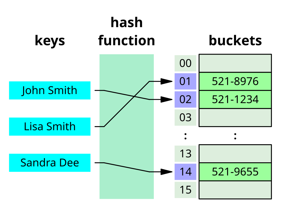
Cost is O(N + M): read each side once. The price is that the first row comes out only after the whole build side has been read. Postgres's code for this, nodeHashjoin.c, is a state machine, and the names of its states describe the same steps as the animation: HJ_BUILD_HASHTABLE reads the build input to the end, HJ_NEED_NEW_OUTER pulls one probe row and hashes its key, and HJ_SCAN_BUCKET compares it against the rows in its bucket and emits each match.
What if the hash table doesn't fit in memory? Its budget is work_mem × hash_mem_multiplier, and work_mem is the memory a single sort or hash is allowed to use before it spills to temporary files (4 MB by default, times 2 for hashes in Postgres 16). When the build side is bigger than that, Postgres splits both inputs into batches by hash value, keeps the first batch in memory, and writes the others to temporary files. Rows can only match rows in their own batch, so when the first batch is done, HJ_NEED_NEW_BATCH loads the next pair of batches from disk, and the build and probe repeat. You can see the cost by squeezing the budget. Joining all 5 million orders to 100,000 customers, one run each:
work_mem | Buckets | Batches | Hash memory | Execution time |
|---|---|---|---|---|
| 4 MB (default) | 131,072 | 1 | 4,540 kB | 1,001 ms |
| 256 kB | 16,384 | 16 | 350 kB | 1,333 ms |
With the smaller budget the hash table gets about a thirteenth of the memory (350 kB instead of 4,540 kB), the inputs are split into 16 batches, and the join takes about a third longer, 1.3 seconds instead of 1.0, because the rows of 15 of the 16 batches are written to temporary files and read back.
5.3Merge join
If both inputs are sorted on the join key, there's a third way. Walk the two inputs side by side like the zip of a jacket, advancing whichever side is behind. In our toy, customers sorted by id and orders sorted by customer_id would be matched in a single pass over each. That's O(N + M) after sorting, with almost no memory. It wins when the sort is free, because both sides come from indexes on the join key, or because the query needs that order anyway for ORDER BY or GROUP BY.
5.4All three, measured
How much does the choice matter? Here's the same join, customers to orders on customer_id, at three sizes, with the planner forced into each algorithm in turn. The runs were warm, in two rounds (medians of three, then of five), and where the rounds differed, both are shown:
| Query | Nested loop (index) | Hash join | Merge join | Planner picked |
|---|---|---|---|---|
| 10 customers (~500 orders) | 0.3 ms | 200–284 ms | 0.2–0.3 ms | Nested loop |
| 2% of customers (~100k orders) | 156–166 ms | 264–490 ms | 6.1–8.2 s | Hash join |
| All 5M orders | 6.8–12.1 s | 0.6–1.4 s | 5.8–11.0 s | Hash join |
| Algorithm | Needs | Cost | Memory | Wins when |
|---|---|---|---|---|
| Nested loop | Nothing (index on inner side to be fast) | N × probe | None | Outer side is small; non-equality joins |
| Hash join | An equality condition | N + M, build first | Build side in memory, or batches | Both sides large and unsorted |
| Merge join | Inputs sorted on the key | N + M plus any sorts | Very little | Inputs already sorted, or output order needed |
Look at the first row. For 10 customers the nested loop took 0.3 ms and the hash join took 200 to 284 ms, because a hash join reads all of one side before it can start, and here that means scanning the orders to find 500 of them. Look at the last row. For all 5 million orders the nested loop took 7 to 12 seconds and the hash join about a second. No algorithm wins everywhere. The planner has to choose by size, which means by estimates.
Now look at the middle row. At 2% of customers the nested loop was faster, 156 to 166 ms against 264 to 490 ms, and yet the planner picked the hash join. The planner chose a plan that was slower, and to find out why we have to look at how it puts a price on each plan.
06How the planner prices a plan
6.1The cost model
Plans are compared by a single number, the cost, and the number is simpler than it looks. It's measured in units of one sequential page read: reading one page of a table in order costs 1.0. Five constants turn every other kind of work into those units:
| Setting | Default | Charged for |
|---|---|---|
seq_page_cost | 1.0 | Each page read in order |
random_page_cost | 4.0 | Each page read out of order |
cpu_tuple_cost | 0.01 | Each row processed |
cpu_index_tuple_cost | 0.005 | Each index entry processed |
cpu_operator_cost | 0.0025 | Each operator or function evaluated |
One word in that table means something new. In cpu_operator_cost, an operator is a single comparison or calculation inside an expression, such as the > in amount > 500, which is a different thing from the plan nodes we've been calling operators. A sequential scan's cost is its page count times seq_page_cost, plus its row count times the per-row CPU cost. Here is that formula in Postgres's source:
	/*
	 * disk costs
	 */
	disk_run_cost = spc_seq_page_cost * baserel->pages;

	/* CPU costs */
	get_restriction_qual_cost(root, baserel, param_info, &qpqual_cost);

	startup_cost += qpqual_cost.startup;
	cpu_per_tuple = cpu_tuple_cost + qpqual_cost.per_tuple;
	cpu_run_cost = cpu_per_tuple * baserel->tuples;
You can check it by hand. The first query below reads the page and row counts the planner has stored for orders, and the other two ask for the plans of a plain scan and a scan with a filter. If the formula is right, we can recompute both costs from the first query's numbers.
select relpages, reltuples from pg_class where relname = 'orders';
explain select * from orders;
explain select * from orders where amount > 500; relpages | reltuples
----------+-----------
41667 | 5000040
Seq Scan on orders (cost=0.00..91667.40 rows=5000040 width=35)
Seq Scan on orders (cost=0.00..104167.50 rows=2500785 width=35)
Filter: (amount > '500'::numeric)Plan one costs 41,667 pages × 1.0 + 5,000,040 rows × 0.01 = 91,667.40, exactly what EXPLAIN printed. That filter in the second query is one operator evaluated per row, so it adds one cpu_operator_cost for each row, 5,000,040 × 0.0025 = 12,500.10, which gives 104,167.50, again exactly. Notice that reltuples, the planner's stored row count, is 5,000,040 and the true count is 5,000,000, so even this number is an estimate, 40 rows off. Index scans, joins and sorts have longer formulas, and an index scan uses the column's correlation to interpolate between random and sequential page costs, but they're all built from these five constants and row estimates.
6.2Why the planner picked the slower join
Back to the 2% query. The planner didn't run the nested loop, it priced it. A nested loop with an index does about 2,000 probes, one for each customer, and each probe fetches heap pages in random order, so each is charged at random_page_cost, which is 4.0 by default. Adding it all up, the nested loop came to a cost of 178,860 against 106,804 for the hash join, so the hash join looked cheaper and won. With random_page_cost set to 1.1 the nested loop was priced at 53,526 and the planner chose it.
Neither price is wrong on its own terms. The setting is a statement about the hardware, and the default describes a disk where random reads are expensive. The Postgres docs say so directly: "Random access to durable storage is normally much more expensive than four times sequential access. However, a lower default is used (4.0) because the majority of random accesses to storage, such as indexed reads, are assumed to be in cache." For a database that fits in memory they advise lowering it: "if your data is likely to be completely in cache, such as when the database is smaller than the total server memory, or network latency is high, decreasing random_page_cost might be appropriate", and "in a heavily-cached database you should lower both values relative to the CPU parameters". Our test database was entirely in memory, so 4.0 overstated the cost of the random probes and the planner talked itself out of the faster plan.
Constants are set once and describe the machine. What changes from query to query is the other input to every formula: how many rows each node will see. The planner has to guess that without looking, and that's where it goes wrong most often.
07Where the row estimates come from
7.1Statistics
Every price in the last section was a number of pages or rows multiplied by a constant. The constants are fixed. The row counts are predictions, and they come from pg_statistic, the catalog table that ANALYZE fills in. ANALYZE doesn't read the whole table. It reads a random sample of 300 × default_statistics_target rows, and since that setting is 100 by default, the sample is 30,000 rows. From the sample it works out, for each column, a few summary figures. The two that do most of the work are a list of the most common values with how often each occurs, and a histogram: a list of values that cut the remaining rows into 100 groups holding the same number of rows each. Here is everything pg_statistic keeps per column, with the values for orders:
| Statistic | What it's for | For orders |
|---|---|---|
null_frac | Fraction of NULLs | 0 everywhere |
n_distinct | Number of distinct values; negative means a fraction of rows | status: 2; r: −0.16 (about 16% of rows distinct) |
most_common_vals / freqs | Up to 100 most common values and their frequency | status: {done, pending} at {0.999, 0.001} |
histogram_bounds | Values splitting the rest into equal-population buckets | 101 bounds for r, id, customer_id |
correlation | Physical order vs sort order (section 4.3) | id: 1; r: −0.004 |
For status = 'pending' the planner reads 0.001 from the most-common-values list and estimates 5,000 rows, which was exactly right. For r < 50000 it finds which group of the histogram 50,000 falls in, counts the full groups below it, and assumes the values inside that one group are spread evenly to estimate the part of it that matches.
7.2Combining predicates: the independence assumption
Our query has a single condition on country, which the statistics handle well. The trouble starts with two conditions. For a WHERE with two of them, the planner multiplies their selectivities, the fraction of rows each keeps. That is only right if the two columns are independent, and real data rarely is. The real customers table has one more column we haven't used, city, with 1,000 different cities spread over the 50 countries, about 100 customers in each city. Each city belongs to exactly one country, so a condition on country that comes with a condition on city removes nothing the city hasn't already removed.
This experiment asks for the customers in city_7 and country_7, with explain analyze, which runs the query and prints the estimated and the actual row count side by side. Then it adds extended statistics, a statistic over a pair of columns that records one determines the other, and asks again:
explain analyze select * from customers
where city = 'city_7' and country = 'country_7';

create statistics cust_city_country (dependencies) on city, country from customers;
analyze customers;

explain analyze select * from customers
where city = 'city_7' and country = 'country_7'; Seq Scan on customers (cost=0.00..2236.00 rows=2 width=26) (actual rows=100 loops=1)
Seq Scan on customers (cost=0.00..2236.00 rows=100 width=26) (actual rows=100 loops=1)Compare rows= with actual rows= in each plan. Without extended statistics the estimate is 100,000 × 1/1,000 × 1/50 = 2 rows, against 100 real ones. With a functional-dependency statistic, the estimate is exact. The view pg_stats_ext showed what ANALYZE had recorded: {"2 => 3": 1.000000}, which means that column 2 (city) determines column 3 (country) in every sampled row.
?Why does a 50× error on one table matter so much?
Because it multiplies up the plan. Joining those customers to a 2-million-row visits table, the planner estimated 1 joined row; there were 36. Every node above it inherits the error. On a bigger query, an estimate of 1 is exactly what makes a nested loop without an index look free.
Leis and colleagues measured how often this happens in their VLDB 2015 study of query optimizers, with 113 multi-join queries over the IMDB data set. They found "all estimators routinely produce large errors", that estimates tend to be systematic underestimates, and that most of Postgres's very slow plans had one thing in common: a nested-loop join without an index. Databases call a node's row count its cardinality, and the paper says Postgres chose those joins "because of a very low cardinality estimate". When the authors disabled such joins, none of their queries timed out any more. They also found the cost model mattered much less than the cardinality estimates.
Even with good estimates, a query with several joins raises one more question. Pricing one join is a formula, but with more than two tables, the planner also has to decide which tables to join first.
08Choosing the join order
With the access paths and join algorithms priced, the planner still has to decide the order. Joining three tables A, B and C could mean (A with B) then C, or (B with C) then A, and so on. For n tables there are n! orders of a left-deep tree alone, a tree in which each join takes one new table: 120 for five tables, over 3.6 million for ten. Pricing millions of plans, each with its own access paths and join algorithms, could easily take longer than running the query.
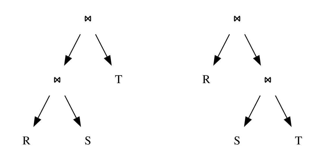
8.1Dynamic programming, from System R
Selinger and colleagues' Access Path Selection paper (SIGMOD 1979) for System R introduced the method nearly every planner still uses: build the best plan for each set of tables bottom up, reusing the best plan for each smaller set. Here's how it plans A ⋈ B ⋈ C, where ⋈ means join:
?Why keep a plan that isn't the cheapest?
Selinger called them interesting orders. A merge join that's slightly more expensive than a hash join, but produces rows sorted by the key a later ORDER BY or merge join needs, can save a sort further up. So the planner keeps the cheapest plan for each useful output order, not just the cheapest overall.
8.2When there are too many tables
2ⁿ still explodes: 4,096 subsets for twelve tables, a million for twenty. Postgres counts FROM items, the tables and subqueries listed in a query's FROM clause, and searches exhaustively when there are fewer than geqo_threshold (12) of them. At 12 or more it switches to a genetic algorithm, a randomised search that evolves a good order without proving it's the best, trading plan quality for planning time. Separately, when a query spells out its joins with explicit JOIN clauses, Postgres won't reorder them if that would mean combining more than join_collapse_limit (8) items.
| Setting | Default | Effect |
|---|---|---|
geqo_threshold | 12 | At this many FROM items or more, use the genetic optimizer |
from_collapse_limit | 8 | Merge subqueries into the parent FROM list only up to this size |
join_collapse_limit | 8 | Reorder explicit JOINs only up to this size; 1 means "join in the order written" |
Everything so far assumed the planner runs once for every query. Planning isn't free, and applications run the same query thousands of times with different values, so the next idea is to plan once and reuse the plan.
09Plans that get reused
Planning costs time, so a prepared statement can reuse its plan. That is a query the application sends once with placeholders (WHERE country = $1) and then runs many times with different values. The catch is that a reused plan was chosen without knowing which value will come next.
9.1Custom and generic plans
Postgres plans the first five executions of a prepared statement with the actual parameter values (custom plans). After that it also builds one generic plan for unknown values, and uses it whenever it's no more expensive than the average custom plan:
	/* Generate custom plans until we have done at least 5 (arbitrary) */
	if (plansource->num_custom_plans < 5)
		return true;

	avg_custom_cost = plansource->total_custom_cost / plansource->num_custom_plans;

	/*
	 * Prefer generic plan if it's less expensive than the average custom
	 * plan.  (Because we include a charge for cost of planning in the
	 * custom-plan costs, this means the generic plan only has to be less
	 * expensive than the execution cost plus replan cost of the custom
	 * plans.)
	 */
	if (plansource->generic_cost < avg_custom_cost)
		return false;

return true;?How does that go wrong?
With skewed data, where a few values are very common and the rest are rare. If the first five executions all use common values and the generic plan matches them, the generic plan wins and is used from then on, including for the rare value where a different plan would be a thousand times faster, or the reverse. The symptom is a query that's fast in psql, Postgres's command-line client, and slow from the application, which uses prepared statements through its driver. plan_cache_mode = force_custom_plan for that statement or session is the direct fix.
That completes the path from text to rows, and each step has shown a place where a plan can go wrong. The last section turns them into a routine for when a query is slow.
10Reading plans on a Monday
10.1What to run
Each question this chapter raised has a command that answers it on a running database.
-- What did it choose, and what did it expect? (sections 2 and 7)
explain select ...;

-- The plan that ran, with real row counts, time and buffers per node (section 7)
explain (analyze, buffers) select ...;

-- For writes, wrap it so nothing changes
begin; explain (analyze, buffers) update ...; rollback;

-- Which queries cost the most in total
create extension pg_stat_statements;
select calls, round(total_exec_time) as ms, round(mean_exec_time, 2) as mean_ms, left(query, 60)
from pg_stat_statements order by total_exec_time desc limit 10;

-- Log plans of slow queries automatically, as the application ran them (section 9)
load 'auto_explain';
set auto_explain.log_min_duration = '500ms';
set auto_explain.log_analyze = on;
When you read an EXPLAIN ANALYZE, work through the same four questions:
- Where's the time? Find the node whose actual time jumps. Remember that
actual timeandrowsare per loop: multiply byloops. - Is any estimate off by 10× or more? Compare
rows=estimated with actual, from the bottom up. The lowest bad estimate is the cause; the ones above it inherit it. - What did it read?
Buffers: shared hitcame from memory,readfrom the operating system,tempmeans a sort or hash spilled to disk. - Would another plan win? Toggle
enable_nestloop,enable_hashjoinorenable_seqscanin a session and compare. That's a diagnosis tool, not a production setting.
10.2Rules that hold up
- Look at the row estimates before anything else. A wrong estimate at the bottom of a plan produces wrong choices all the way up.
- Run
ANALYZEafter a big change to a table, and add extended statistics for columns that depend on each other. - Set the cost constants to match your hardware. On SSDs, or when the data fits in memory, lower
random_page_cost. - Build composite indexes in the order equality columns, then one range column, and check them with
EXPLAIN. - Use
EXPLAIN (ANALYZE, BUFFERS)on the query as the application ran it, with the same parameters, in the same session settings.
10.3What you trade for what
| You get | You pay | When the bill arrives |
|---|---|---|
| Row-at-a-time execution that composes | Per-row overhead on big scans | As a dashboard query that's 18 times slower than a vectorized engine |
| A plan chosen from statistics before reading data | A plan is only as good as its estimates | As a query that takes 30 seconds instead of 5 ms |
| An index on every filtered column | Every INSERT and UPDATE maintains each index | As slow writes |
| A reused plan with no planning cost | The plan was chosen without the value | As a query that's fast in psql and slow from the app |
| Exhaustive join ordering | Planning time that grows as 2ⁿ | As a switch to a genetic search at 12 tables |
10.4Symptom, cause, fix
| Symptom | Likely cause | Fix |
|---|---|---|
Nested loop with loops= in the thousands and a huge actual row count | Outer side underestimated | Fix statistics (ANALYZE, higher target, extended stats); check correlated predicates |
| Seq scan on a big table for a selective filter | No suitable index, a function on the column, or a type mismatch | Composite or expression index; compare like types |
| Index scan slower than expected on a large range | Low correlation; rows scattered | Let it use a bitmap scan; CLUSTER for read-mostly tables; a covering index |
Sort Method: external merge or hash Batches above 1 | work_mem too small for this node | Raise work_mem for that session or query, not globally |
Fast in psql, slow from the app | Generic plan from a prepared statement | plan_cache_mode = force_custom_plan for it |
| Plan changed overnight and got slow | Statistics changed after autovacuum's ANALYZE, or data crossed a threshold | Compare old and new plans with auto_explain; fix the estimate |
| Planner prefers seq scans on an SSD box where indexes are faster | Default random_page_cost = 4 | Lower it towards 1.1 for SSD or fully cached data |
| Big ORM query with an odd join order | More tables than join_collapse_limit | Raise the limit, or simplify the query |
11Summary
- A query says what and never how. The database parses, analyses, rewrites, plans and executes it, and only the executor reads data. The planner decides everything before that, from statistics.
- A plan is a tree of operators, and
EXPLAINprints it with estimated cost and rows for each node. - Row stores run plans one row at a time. The Volcano model composes well, but per-row overhead dominates big scans: Postgres spent 29 ns a row where DuckDB spent 1.6.
- Index scans pay per row, sequential scans per page. On a random column the crossover was near 3% of rows, and bitmap scans cover the middle ground by visiting each page once.
- Correlation decides how bad an index scan gets. On a column matching disk order, the index scan still won at 50%.
- Nested loop wins with a small outer side and an index. It took 0.3 ms against 200 ms for a hash join on ten customers.
- Hash join wins when both sides are big. 5M rows joined in about a second, against 6 to 12 seconds for the others.
- Cost is pages plus rows times five constants. A Seq Scan on
orderscosts exactly 41,667 + 5,000,040 × 0.01. - The defaults assume slow random I/O. Lowering
random_page_costflipped a join to the faster nested loop. - Row estimates are the usual culprit. Multiplying correlated predicates turned 100 rows into an estimate of 2, and extended statistics fixed it.
- Join order is dynamic programming over subsets below 12 tables, with a genetic search from 12 up and no reordering of explicit joins past 8, and a reused plan can be wrong for the next value.
12Build this
A query engine you can read in an afternoon.
- Implement Volcano operators over in-memory rows:
Scan,Filter,Project,NestedLoopJoin,HashJoin,Sort,Limit, each withnext(). Check thatLimitstops the scan early. - Rewrite
Scan,Filterand aSumaggregate to pass batches of 1,024 values in columnar arrays. Time both on 10 million rows and compare your ns per row with the 29 and 1.6 from section 3.4. - Add a planner for three-table joins: estimate each filter's selectivity from a histogram, enumerate join orders by dynamic programming, and pick nested loop or hash join by a cost formula. Then feed it correlated columns and watch it choose badly.
13Interview questions
beginnerWhat's the difference between EXPLAIN and EXPLAIN ANALYZE?›
EXPLAIN shows the chosen plan with estimated costs and row counts, without running it. EXPLAIN ANALYZE runs the query and adds actual time, actual rows and loops per node, and with BUFFERS, the pages read. For a write, it performs the write, so wrap it in a transaction and roll back.
beginnerWhen would a database choose a sequential scan even though an index exists?›
When enough rows match that visiting them through the index costs more than reading every page in order. On a random column that happened near 3% of rows in memory, and much earlier on disk. Also when the table is small, or the statistics say the value is very common.
intermediateDescribe hash join, nested loop and merge join, and when each wins.›
Nested loop probes the inner side once per outer row. With an index on the inner key it's best for a small outer side, and it's the only one that handles non-equality joins. Hash join builds a hash table on the smaller side and probes it with the larger, O(N + M), best for large unsorted equi-joins, spilling to batches if the build side exceeds memory. Merge join walks two sorted inputs in step. It wins when both are already sorted or the output order is needed.
intermediateA query's EXPLAIN ANALYZE shows rows=1 estimated and rows=50000 actual at a scan. What do you do?›
Treat it as the cause, since everything above it inherits the error. Check when the table was last analysed, and run ANALYZE. If the filter combines correlated columns, add extended statistics (CREATE STATISTICS … (dependencies)). If the column is skewed, raise its statistics target. Then check that the plan changed, typically from a nested loop to a hash join.
intermediateWhat's the difference between Volcano and vectorized execution?›
Volcano operators return one row per next() call, with interpreted expressions, so per-row overhead (calls, interpretation, row-format access) dominates big scans. Vectorized operators pass batches of roughly a thousand values per column, paying that overhead once per batch and running tight loops the compiler can turn into SIMD. On the same 5M-row aggregate, Postgres took 145 ms on one core and DuckDB 8 ms on one thread, helped by columnar storage too.
deepHow does a planner choose a join order for eight tables without trying 40,320 orders?›
Dynamic programming over subsets, from System R: find the best plan for each single table, then each pair, then each triple, always building from the best plans of smaller subsets, so each subset is solved once. That's about 2ⁿ subsets instead of n! orders. It keeps extra plans for interesting sort orders. Postgres does this below geqo_threshold (12) tables, then switches to a genetic search, and doesn't reorder explicit joins beyond join_collapse_limit (8).
deepWhy is a query fast in psql but slow from the application?›
Often a prepared statement. The driver prepares it, Postgres plans the first five executions with real parameter values, then switches to a generic plan if it's no costlier than their average. With skewed data the generic plan can be terrible for some values. Check with EXPLAIN (ANALYZE) EXECUTE after six executions, or with auto_explain, and use plan_cache_mode = force_custom_plan. Other causes are different settings (work_mem, search_path) or a different parameter type causing a cast that disables an index.
14Go deeper
A table has 1,000 pages and 100,000 rows. What does the planner charge for a Seq Scan with one filter?›
1,000 × 1.0 + 100,000 × (0.01 + 0.0025) = 2,250.
Why does a bitmap heap scan beat a plain index scan at 5% on a random column?›
It collects all matching TIDs first and sorts them by page, so each heap page is read once and in order instead of once per matching row.
Two predicates each keep 10% of rows. What does Postgres estimate for both together?›
1%, by multiplying, unless extended statistics say the columns are dependent.
What does a hash join do when the build side doesn't fit in work_mem × hash_mem_multiplier?›
Splits both inputs into batches by hash value, keeps one batch in memory, writes the rest to temporary files and processes them one pair at a time.
The System R optimizer: cost formulas, selectivity estimates, dynamic programming over join orders and interesting orders.
The iterator model almost every row store still uses, plus the exchange operator for parallelism.
Why tuple-at-a-time engines waste the CPU, and the vectorized design that became Vectorwise and inspired DuckDB.
Data-centric code generation with LLVM, the design behind HyPer and Umbra.
The Join Order Benchmark, and measurements showing cardinality estimates, not cost models, cause most bad plans.
Section 14.1 and chapter 76: every field in a plan, and worked examples of the selectivity arithmetic with MCVs and histograms.
15Related chapters
The B+tree pages an index scan walks, the heap it visits, and the buffer pool rings that keep a Seq Scan from flushing the cache. Chapter 18.
Why a Seq Scan takes a relation-level SIREAD lock under serializable, and what the visibility checks on every row cost. Chapter 19.
Branch prediction, SIMD and instruction-level parallelism: the hardware reasons vectorized execution is faster. Chapter 01.
Why a columnar batch that fits in L1 beats a row scattered across a page. Chapter 02.