Priya steps out of Pune railway station with a suitcase and opens the Uber app. The map already shows a handful of small cars crawling along the streets around her. She sets the airport as her destination, taps Request, and within a couple of seconds the screen says that Ravi, in a white hatchback, is three minutes away. She watches the little car turn two corners and pull up beside her.
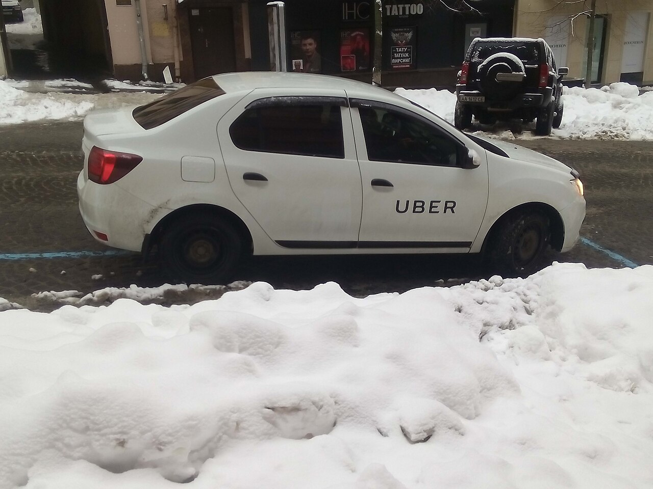
It looks like a simple lookup, "find the nearest car", but almost every word in that phrase hides a problem. The cars are moving, so wherever the system thinks Ravi is, he was there a few seconds ago. There are millions of them worldwide, so checking every car for every request is out of the question. "Nearest" in a straight line can mean a car on the far side of a river, ten minutes away by road. And picking the nearest car for Priya might leave the rider who taps Request one second later with a car twice as far away, when a slightly different pairing would have suited both.
In this case study we'll design the system that answers Priya's request, the way an engineer would: start with the most obvious design, find exactly where it breaks, and fix it, step by step. The question we'll keep coming back to is this: when Priya taps Request, how does Uber pick the right car out of millions of moving ones, in a second or two? Along the way we'll go from boxes on a diagram down to hexagonal grids, 64-bit cell IDs, road graphs and an assignment problem.
01What we're building, and how big
1.1What it has to do
The core of Uber, the part that moves people, comes down to a short list:
- Show nearby cars on the rider's map as soon as the app opens.
- Match a request to a driver, and get the driver to accept it.
- Estimate times: how long until the car arrives, and how long the trip will take.
- Price the trip, including raising prices where demand outruns supply (surge).
- Track the trip live for both rider and driver, from pickup to drop-off.
- Charge the rider and pay the driver once the trip ends.
And the qualities it needs while doing that:
- Fresh: the system's idea of where each car is should be seconds old, not minutes.
- Fast: a match within a couple of seconds of tapping Request.
- Correct where it matters: one driver can't be assigned to two riders at once, and a trip that has started must never be forgotten.
- Available: a failing data centre mustn't strand riders mid-trip.
This list differs from WhatsApp's in one important way. WhatsApp's hard problem was delivering messages to the right place; Uber's is a question about space: which of the moving things are close to this point, and in what sense of close. Most of this case study is about answering that question quickly.
1.2How big is it?
Uber's own filings give the scale. In the quarter that ended in June 2026, the platform handled about 3.9 billion trips and had 208 million people using it each month. A record 10.2 million drivers and couriers earned money on it that quarter. Across 2025, Uber completed about 13.6 billion trips, more than 40 million a day. (These "trips" include food and package deliveries, not only rides.) It operates in over 70 countries and more than 15,000 cities.
The number that shapes the design most, though, is how often each car reports where it is. Every driver's phone works out its position from GPS satellites and sends it to Uber's servers every few seconds. Uber described this in 2015 as every four seconds, and its partner API still delivers driver locations at a four-second interval by default.
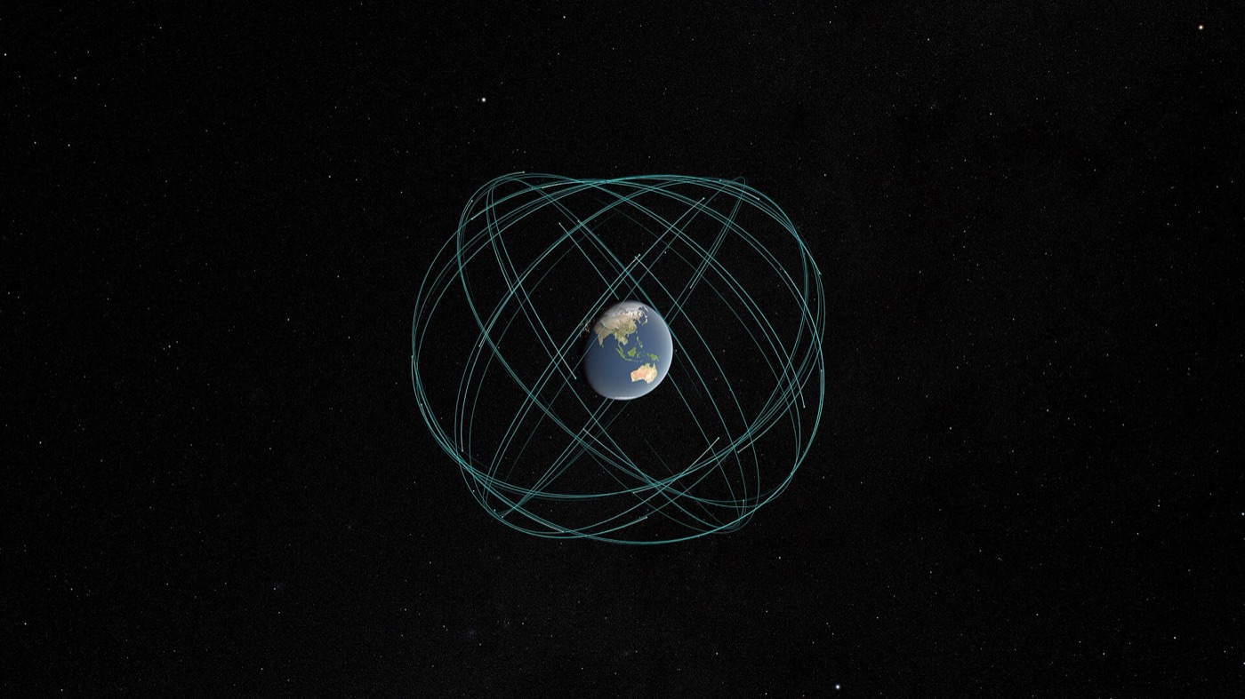
Suppose a million drivers are online at the same moment, each sending a location every four seconds. How many location updates arrive per second, and how long is each one worth keeping?
02Version 1: a table of drivers
2.1The obvious design
The most obvious design is a database table with one row per driver: driver ID, latitude, longitude, and whether they're free. Each location update overwrites the driver's row. When Priya requests a ride, the server asks for the free drivers ordered by distance from Priya and takes the closest.
Both halves break at Uber's scale. The writes are the first problem: a quarter of a million updates a second to a database on disk, each one written durably even though it will be useless four seconds later. The reads are the second: "order by distance from Priya" means computing the distance from Priya to every free driver and sorting. An ordinary database index can't help, because an index sorts by one value, and distance from Priya isn't a value stored in any row; it depends on where Priya is.
So we need two things: a place to keep the latest positions that can absorb constant overwrites, and a way to find the drivers near a point without looking at all of them. The first is the easy part. Since only the latest position matters and it's replaced every few seconds anyway, it can live in memory. The rest of this section's trouble, finding nearby drivers without scanning everyone, takes the whole of the next section.
03Finding what's nearby: indexing space
3.1Chop the map into cells
Here's an idea you'd probably come up with yourself. Divide the city into a grid of squares, say 500 metres on a side, and keep a list of the drivers currently inside each square. When Ravi's update arrives, compute which square he's in (divide his coordinates by 500 and round down) and move him into that square's list if he's crossed a line. When Priya requests, look only in her square and the eight squares around it.
This program tries it with a million drivers scattered over a 40 km by 40 km city, comparing it with checking every driver:
import math, random, time
random.seed(1)

# 1,000,000 drivers scattered over a 40 km x 40 km city
N, SIZE = 1_000_000, 40_000.0
drivers = [(random.uniform(0, SIZE), random.uniform(0, SIZE)) for _ in range(N)]
rider = (21_345.0, 18_210.0)

def dist(a, b):
    return math.hypot(a[0] - b[0], a[1] - b[1])

# 1. brute force: look at every driver
t = time.perf_counter()
best = min(drivers, key=lambda d: dist(d, rider))
brute_ms = (time.perf_counter() - t) * 1000

# 2. grid index: 500 m cells, look only in the rider's cell and its neighbours
CELL = 500.0
grid = {}
for d in drivers:
    grid.setdefault((int(d[0] // CELL), int(d[1] // CELL)), []).append(d)

t = time.perf_counter()
cx, cy = int(rider[0] // CELL), int(rider[1] // CELL)
nearby = [d for dx in (-1, 0, 1) for dy in (-1, 0, 1)
          for d in grid.get((cx + dx, cy + dy), [])]
best_grid = min(nearby, key=lambda d: dist(d, rider))
grid_ms = (time.perf_counter() - t) * 1000

print(f"brute force: {N:,} drivers checked, {brute_ms:.1f} ms")
print(f"grid index:  {len(nearby):,} drivers checked, {grid_ms:.3f} ms")
print(f"same driver found: {best == best_grid}, {dist(best, rider):.0f} m away")brute force: 1,000,000 drivers checked, 81.7 ms
grid index: 1,456 drivers checked, 0.327 ms
same driver found: True, 24 m awayThe grid found the same driver after looking at 1,456 drivers instead of a million, about 250 times faster (the exact times vary from run to run). The program has a deliberate shortcut: it assumes the nearest driver is within one cell of Priya, which is true here because the city is evenly packed with drivers. With sparse drivers, the search has to widen ring by ring until it finds someone.
That last caveat is the grid's real weakness, because real cities are not evenly packed. At 6 pm a 500-metre square in central Mumbai might hold hundreds of cars while one on the outskirts holds none. A single cell size is too coarse downtown, where every cell holds too many cars, and too fine in the suburbs, where Priya's search has to step through many empty cells. The fixes are smarter ways to cut space into cells, and there are four well-known ones.
3.2Geohash: a cell you can write as a string
A geohash turns a location into a short string, by repeatedly halving the world. The first step asks "is the point east or west of the middle longitude?" and records a 1 or a 0. The next asks "north or south of the middle latitude?", and so on, alternating, halving the remaining box each time. Every five of those bits become one character from a 32-character alphabet. Each extra character makes the box 32 times smaller.
BASE32 = "0123456789bcdefghjkmnpqrstuvwxyz"

def geohash(lat, lon, length=7):
    lat_lo, lat_hi, lon_lo, lon_hi = -90.0, 90.0, -180.0, 180.0
    bits, even, out = 0, True, ""
    for i in range(length * 5):
        if even:                      # even bits split longitude
            mid = (lon_lo + lon_hi) / 2
            bit = lon >= mid
            lon_lo, lon_hi = (mid, lon_hi) if bit else (lon_lo, mid)
        else:                         # odd bits split latitude
            mid = (lat_lo + lat_hi) / 2
            bit = lat >= mid
            lat_lo, lat_hi = (mid, lat_hi) if bit else (lat_lo, mid)
        bits = bits * 2 + bit
        even = not even
        if i % 5 == 4:
            out += BASE32[bits]
            bits = 0
    return out

places = {
    "Pune station":   (18.5286, 73.8743),
    "Koregaon Park":  (18.5362, 73.8940),
    "Mumbai CST":     (18.9398, 72.8355),
}
for name, (lat, lon) in places.items():
print(f"{name:14} {geohash(lat, lon)}")Pune station tek93j1
Koregaon Park tek93qr
Mumbai CST te7g9rvPune station and Koregaon Park, about two kilometres apart, share the first five characters, tek93. Mumbai, 120 km away, shares only te. That's the property that makes geohashes useful: nearby places usually share a long prefix, so "drivers near Priya" becomes "drivers whose geohash starts with tek93", a prefix search that any ordinary sorted index, in Redis, Postgres or Cassandra, can answer.
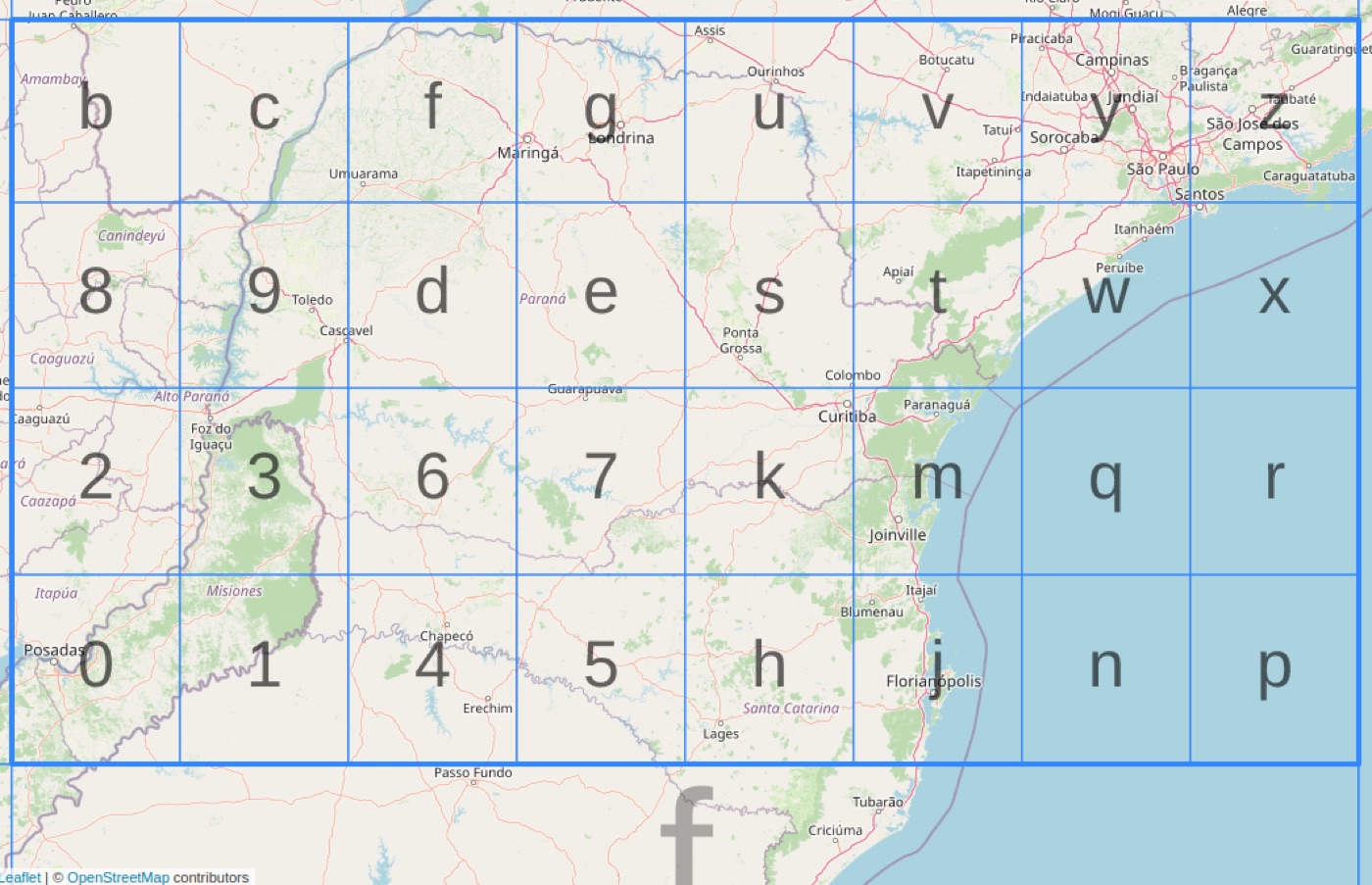
The word "usually" in that paragraph is the catch. The halving traces a zig-zag path through space called a Z-order curve, and where the curve jumps, two points a few metres apart on either side of a cell boundary can have completely different prefixes. A geohash search therefore always has to check the eight neighbouring cells too, just like the grid. Geohash cells also get narrower towards the poles, so a "cell" isn't the same size everywhere.
3.3Quadtrees and S2: cells that adapt
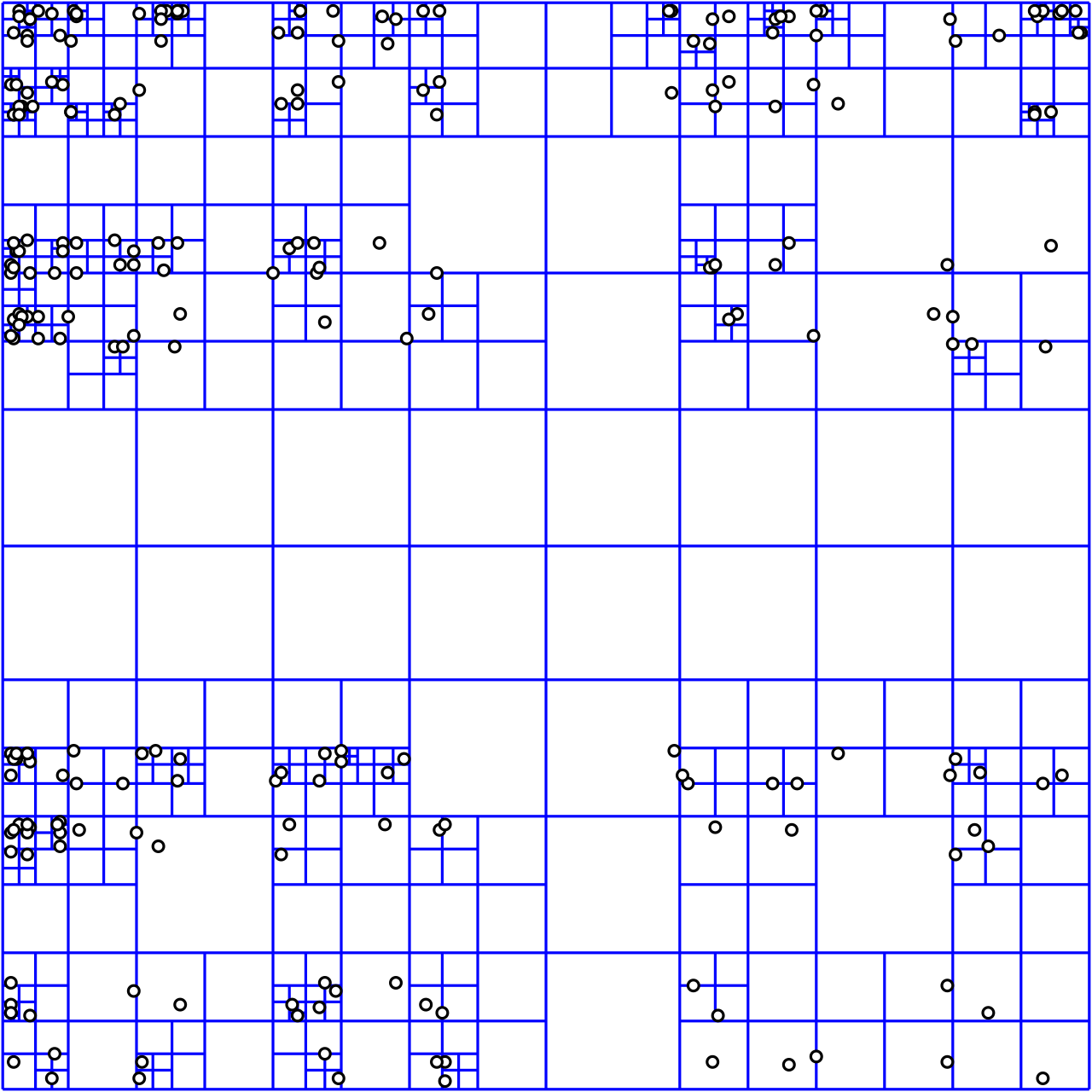
A quadtree fixes the density problem directly. Start with one square covering the city. Whenever a square holds more than some limit of drivers, split it into four equal squares, and keep splitting until every square is below the limit. Busy downtown streets end up covered by many small squares, and empty suburbs by a few big ones.
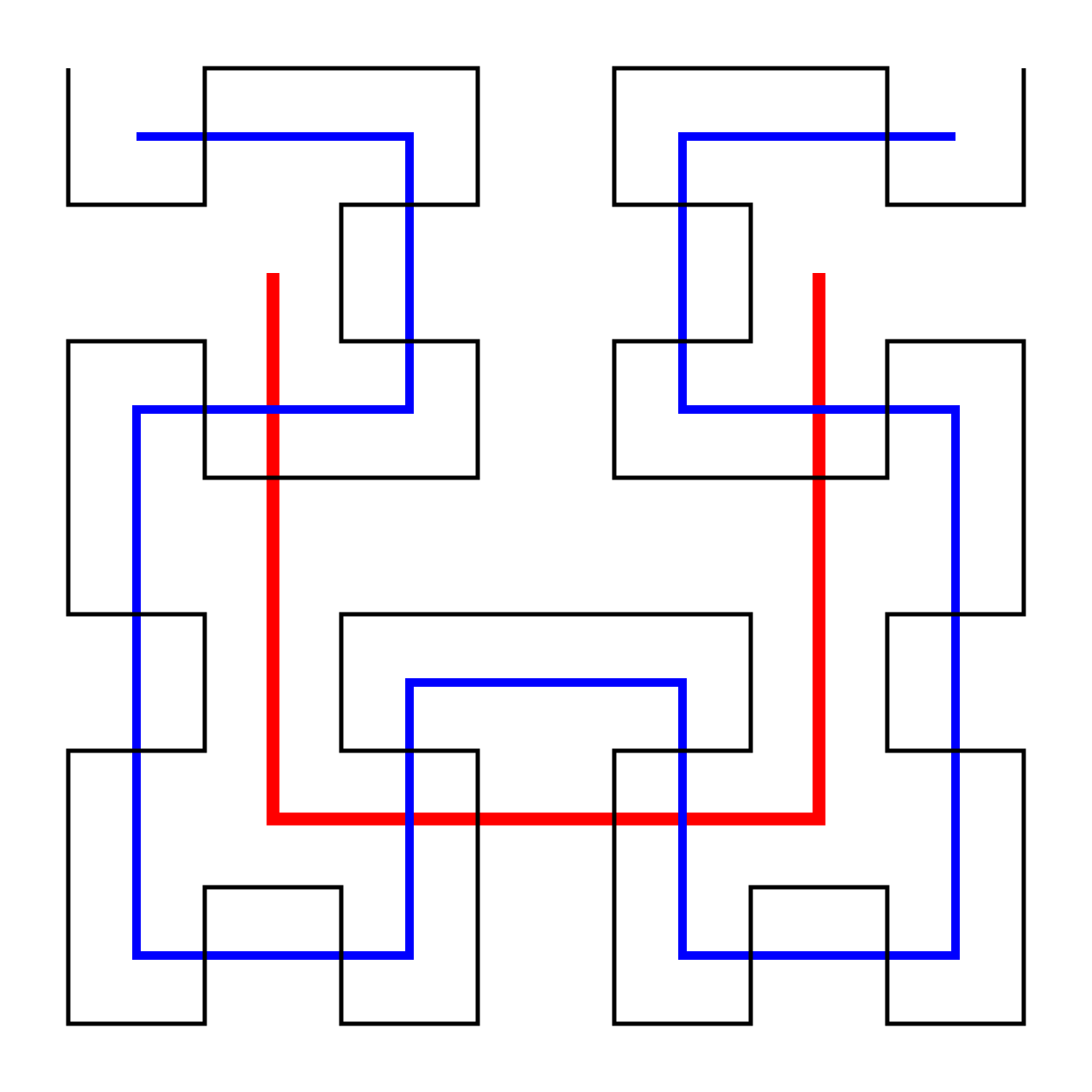
Google's S2 library takes the hierarchy of squares and makes it global and fixed. It projects the Earth onto the six faces of a cube and divides each face into a quadtree of cells, 31 levels deep. Each cell gets a 64-bit ID, numbered along a Hilbert curve, a path that winds through every cell without the big jumps of the Z-order curve. Cells that are close on the curve are close on the ground, so a range of IDs covers a compact area, which suits a sorted index well. According to write-ups of a 2015 Uber talk, Uber's dispatch system used S2 cells at level 12, each a few square kilometres, to organise its driver index at the time.
3.4H3: hexagons
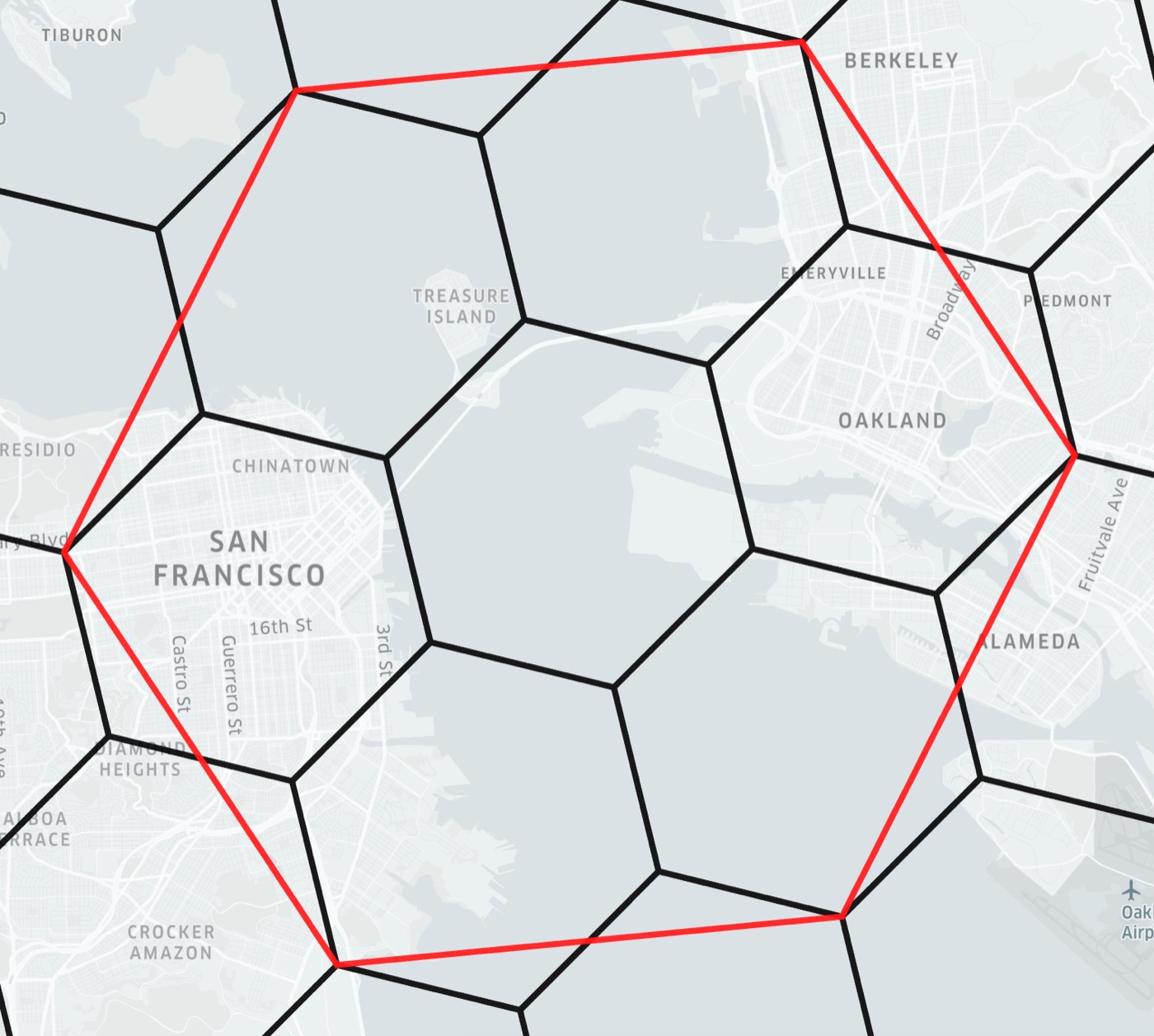
In 2018 Uber open-sourced its own grid system, H3, and it isn't made of squares at all. H3 covers the Earth with hexagons.
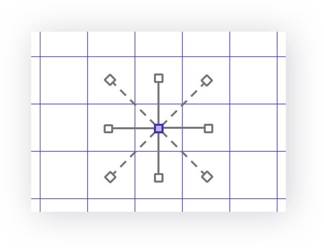
The reason is the neighbours. Look at a square cell: four neighbours share an edge with it, and four more touch it only at a corner, about 1.4 times further away. Any calculation that spreads out from a cell, such as "demand in this area and the areas around it", has to treat those two kinds of neighbour differently. A hexagon has six neighbours, all sharing an edge and all at the same distance. Uber's 2018 post puts it plainly: hexagons have only one distance between a cell's centre and its neighbours', where squares have two.
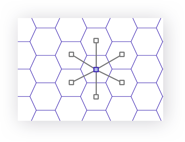
H3 offers 16 resolutions, from cells the size of continents down to cells under a square metre. Each finer resolution has cells about a seventh the area of the one above:
| Resolution | Average cell area | Average edge | Cells on Earth |
|---|---|---|---|
| 0 | 4,357,449 km² | 1,281 km | 122 |
| 7 | 5.16 km² | 1.41 km | about 99 million |
| 8 | 0.74 km² | 0.53 km | about 692 million |
| 9 | 0.11 km² | 0.20 km | about 4.8 billion |
| 15 | 0.9 m² | 0.58 m | about 570 trillion |
A city-scale question uses resolutions around 7 to 9: a resolution-8 hexagon is roughly a neighbourhood, half a kilometre across. Which resolution Uber uses for each job isn't published.
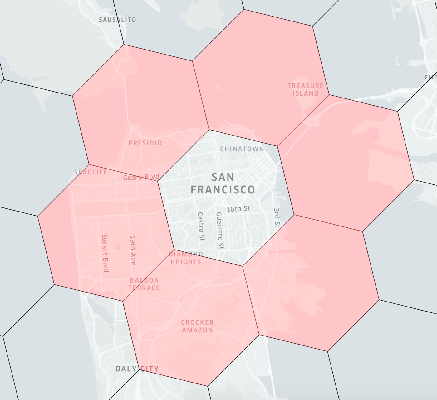
"Find drivers near Priya" in H3 becomes: find Priya's cell, then ask for every cell within k steps of it. That operation is called gridDisk (it was named kRing in earlier versions). With k = 1 it returns Priya's cell and its 6 neighbours, 7 cells. In general it returns 3k² + 3k + 1 cells, so 19 for k = 2, and the search widens ring by ring until enough drivers turn up.
Hexagons have one drawback, and it's built into geometry: you can't divide a hexagon exactly into seven smaller hexagons. H3's children cover their parent only approximately, slightly rotated, where S2's four children tile their parent square exactly.
3.5Inside an H3 cell ID
An H3 cell is identified by a single 64-bit integer, which is what makes it cheap to store, hash and compare. The bits are laid out like this:
| Bits | Field | What it holds |
|---|---|---|
| 1 | reserved | always 0 |
| 4 | mode | 1 means "this is a cell" (other modes encode edges and vertices) |
| 3 | reserved | |
| 4 | resolution | 0 to 15 |
| 7 | base cell | which of the 122 resolution-0 cells it descends from |
| 45 | 15 digits × 3 bits | one digit (0 to 6) per resolution, choosing one of seven children at each step; unused digits are set to 7 |
So an ID is literally a path: start from one of the 122 base cells and take one of seven turns at each resolution. Finding a cell's parent means setting the resolution field one lower and blanking the last used digit, a couple of bit operations. That's also what makes compaction possible: when all seven children of a parent are in a set, replace them with the parent. Uber's 2018 post gives the example of California: 10,633 cells at resolution 6, or 901 cells once compacted into a mix of resolutions.
Which way of cutting the map into cells?
- A plain string: works with any sorted index
- Easy to implement
- Neighbours across boundaries have unrelated prefixes
- Cells shrink towards the poles
- Exact parent-child containment
- Hilbert order keeps ID ranges compact
- Two kinds of neighbour: edge and corner
- Every neighbour at the same distance
- Smooth for spreading and aggregating values
- One 64-bit ID per cell
- Children only approximately fill their parent
- 12 pentagons at every resolution need special care
Uber built H3 because its most demanding spatial questions were about areas, not points: demand and supply per neighbourhood, smoothed across adjacent neighbourhoods for surge pricing, and analysed across a whole city. Equal-distance neighbours make that smoothing simple and unbiased. For pure "which drivers are near this point" lookups, the choice matters less; any of the four works with a neighbour search, which is why Uber's 2015 dispatch system could use S2 cells.
04Keeping the live map of drivers
4.1Too much for one machine
We now know how to find nearby drivers in a grid. The next question is where that grid lives. Holding the latest position of a few million drivers takes only a few hundred megabytes, which fits on one machine easily. The problem is the traffic: a quarter of a million updates a second, plus every rider's search, plus the fact that one machine is one machine, and when it fails, nobody can get a ride anywhere.
So the index is split across many machines, and the natural way to split it is by cell. Each machine owns some set of cells and holds the drivers currently inside them. Ravi's location update goes to whichever machine owns his current cell. Priya's search goes to the machines that own the cells in her gridDisk, usually just one or two, since nearby cells tend to be on the same machine.
One property of this workload makes failures far less painful than usual. Because every driver resends their position every four seconds, a node that crashes and restarts empty is fully repopulated within a few seconds, without any backup or replica. The data heals itself. That's a big part of why it can live in memory at all.
4.2Who owns which cells: Ringpop
Something has to decide which node owns each cell, and keep every node and gateway in agreement as nodes join, crash and restart. Uber built and open-sourced a library for this in 2015 called Ringpop, and the motivating case was exactly this driver-location service.
Ringpop combines two ideas from chapters 29 and 30. The first is a consistent hash ring: each node is placed at several points on a circle of hash values, and each key, here a cell ID, belongs to the first node clockwise from the key's hash. When a node leaves, only its keys move, to its neighbours on the ring; everyone else's stay put. Ringpop keeps the ring in a red-black tree, so finding a key's owner takes a logarithmic number of steps.
The second is SWIM gossip for membership: nodes ping each other at random, ask others to ping a node that doesn't answer, mark it suspect and then faulty, and spread those changes by piggybacking them on their pings. So there's no central coordinator; every node keeps its own copy of the membership list and the copies converge.
When a request arrives at a node that doesn't own the key, that node forwards it to the owner. Uber called this "handle or forward". Any node can take any request, which keeps clients simple.
How do nodes agree on who owns which cells?
- One source of truth
- Easy to reason about
- Another critical system to run
- Every membership change goes through it
- No central component
- Only a failed node's keys move
- Membership views can briefly disagree
- Gossip traffic grows with cluster size
Ringpop fitted 2015's Uber: services written in Node.js, growing fast, without an existing coordination layer. It didn't last everywhere. By 2017 Uber's push platform had replaced Ringpop with Netty, ZooKeeper and Apache Helix, and in 2021 Uber's engineers cited Ringpop's peer-to-peer protocol as one of the limits that led them to rebuild the trip-handling platform. Gossip is excellent at "roughly who is alive"; it's a poor fit when an assignment must be exactly right, which is the subject of section 5.3.
05Choosing a driver
5.1Nearest isn't quickest
Dispatch now has a list of candidate drivers near Priya. The next mistake to avoid is picking the closest one in a straight line. Pune has a river running through it, and the nearest car in a straight line might be across a bridge that's twenty minutes away at rush hour, while a car twice as far away is on Priya's side of the river and three minutes from her.
So matching is done on estimated time of arrival (ETA), computed along the actual road network, not on straight-line distance. Uber's own description of its marketplace says it directly: closest doesn't always mean quickest, because of traffic, overpasses, rivers and other geography. The straight-line search from section 3 still has a job, though. It cheaply narrows millions of drivers down to a few dozen, and only those few dozen get the expensive road-based ETA calculation, which section 6 covers.
5.2One rider at a time, or a batch?
The second mistake is subtler. Suppose two riders request within a second of each other, and two free drivers are nearby.
Priya requests first, then Sam a second later. Ravi is 2 minutes from Priya and 3 from Sam. Meena is 4 minutes from Priya and 9 from Sam. If each rider in turn takes the nearest free driver, what's the total waiting time? Can you do better?
This short program does both: greedy in order of request, and a search over every possible pairing for the lowest total wait.
from itertools import permutations

# minutes for each driver to reach each rider
eta = {
    ("Ravi", "Priya"): 2, ("Ravi", "Sam"): 3,
    ("Meena", "Priya"): 4, ("Meena", "Sam"): 9,
}
riders, drivers = ["Priya", "Sam"], ["Ravi", "Meena"]

# Greedy: each rider, in order of request, takes the nearest free driver
free, greedy = set(drivers), {}
for r in riders:
    d = min(free, key=lambda d: eta[(d, r)])
    greedy[r] = d
    free.remove(d)

# Batched: try every assignment, keep the lowest total wait
best = min(permutations(drivers),
           key=lambda ds: sum(eta[(d, r)] for d, r in zip(ds, riders)))
batched = dict(zip(riders, best))

for name, plan in [("greedy", greedy), ("batched", batched)]:
    waits = {r: eta[(d, r)] for r, d in plan.items()}
print(f"{name:8} {plan} waits {waits} total {sum(waits.values())} min")greedy {'Priya': 'Ravi', 'Sam': 'Meena'} waits {'Priya': 2, 'Sam': 9} total 11 min
batched {'Priya': 'Meena', 'Sam': 'Ravi'} waits {'Priya': 4, 'Sam': 3} total 7 minPairing riders with drivers to minimise the total cost is a classic problem called bipartite matching, or the assignment problem. Trying every pairing, as the program does, works for two riders and two drivers, but the number of pairings grows factorially, so real solvers use algorithms such as the Hungarian algorithm, which solves it in polynomial time, or min-cost flow. Uber hasn't published which solver it uses.
Should each request be matched the moment it arrives?
- The fastest possible answer for each rider
- Trivial to implement
- Early riders can take drivers that later riders needed far more
- Total waiting across everyone is higher
- Lower waiting time across everyone
- Can count drivers who are about to finish a nearby trip
- Each rider waits a few seconds longer for the match
- A heavier computation per batch
Uber's marketplace page describes exactly this: waiting just a few seconds after a request lets it pair riders and drivers to reduce the average wait for everyone, "not just the closest pair". The same window lets the dispatcher consider a driver who is about to drop someone off around the corner, who would be invisible to a search for free drivers only; Uber's dispatch rewrite in 2015 was built to plan ahead in this way.
5.3One driver, one trip
The batch gives Ravi to Sam. Dispatch sends Ravi an offer, Ravi's phone shows it with a countdown, and Ravi taps Accept. If Ravi ignores it, the offer expires and Sam goes back into the next batch.
Here, for the first time, correctness matters more than speed. Two dispatch processes, perhaps handling neighbouring areas, must never offer Ravi to two riders at once, and once Ravi accepts, the trip must exist and be remembered whatever fails. Think of each driver and trip as a small state machine, where only certain moves are allowed, and each move must happen at most once:
The state names here are illustrative; Uber's internal ones aren't public. What is public is how its thinking changed. Uber's original trip platform was built, in its engineers' words, on the premise of trading consistency for availability and latency, using Node.js, Ringpop, Cassandra and Redis. In 2021 Uber described rebuilding it in Java on Google Cloud Spanner, a database that offers transactions across shards, and modelling each driver, rider and trip as a hierarchical state machine. The rebuilt platform served over a million concurrent users in over 10,000 cities.
For driver and trip state, favour availability or consistency?
- Keeps working through partitions and node failures
- Low latency
- Rare double assignments and lost updates to clean up
- Hard-to-reason-about edge cases as products multiply
- A driver can't be in two trips
- Simpler code for complex flows
- A distributed database with higher write latency
- Depends on the database's availability
The location index and the trip state ended up with opposite answers, and that's the right outcome: locations are overwritten every four seconds and heal themselves, so losing one costs nothing; a trip is a promise to a rider and a driver, so losing or doubling one costs a great deal. Chapter 19 covers what "transactions across shards" requires, and chapter 31 what it costs.
06How long will it take?
6.1The road network as a graph
Matching needs an ETA for each candidate driver, and the app shows ETAs all the time: for the car to arrive, for the trip, for the price estimate. To compute one, Uber models the road network as a graph: every intersection is a node, every stretch of road between two intersections is an edge, and each edge's weight is how long it takes to drive. Turn restrictions and the cost of turning are modelled too. An ETA is then the length of the shortest path between two nodes.
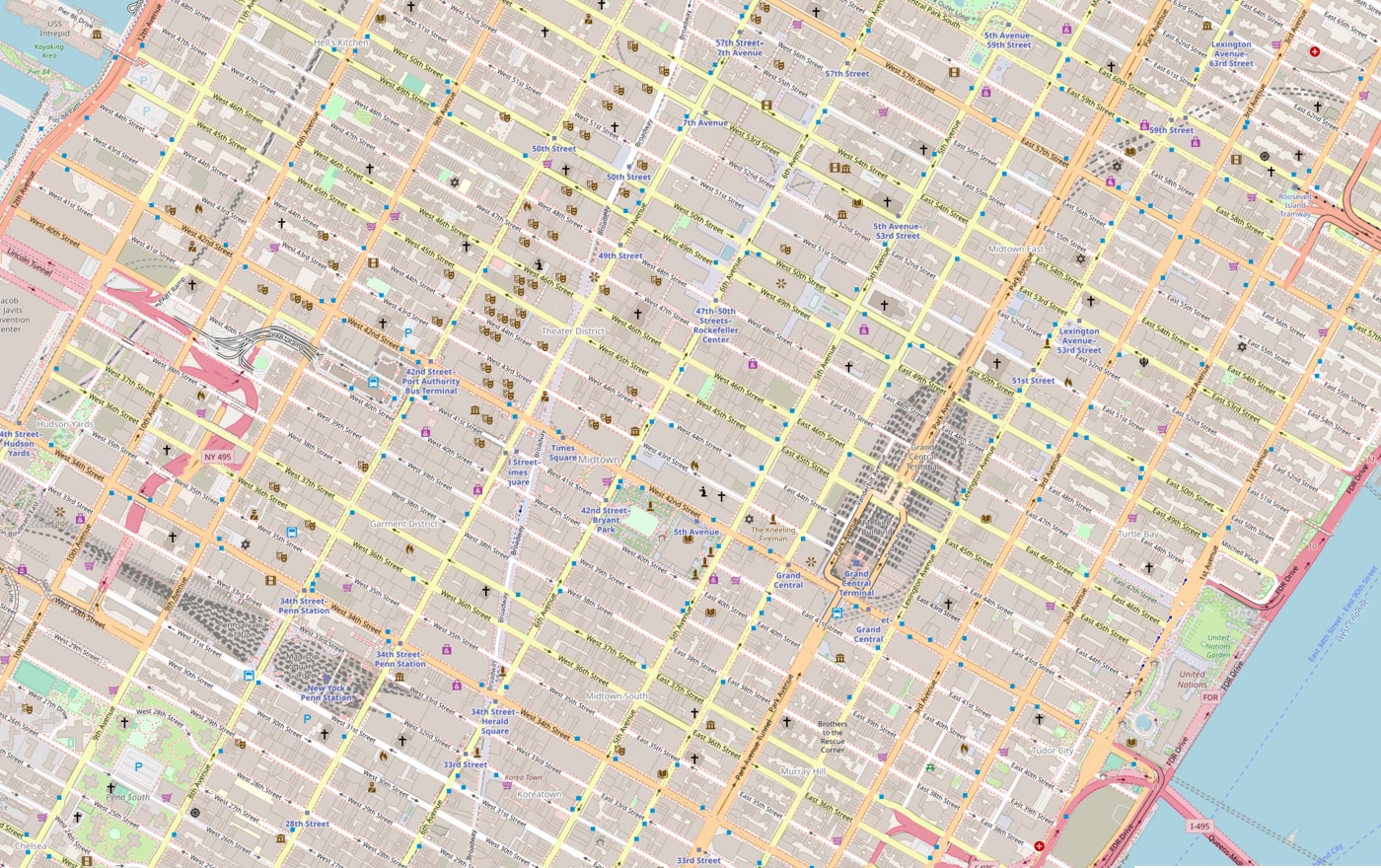
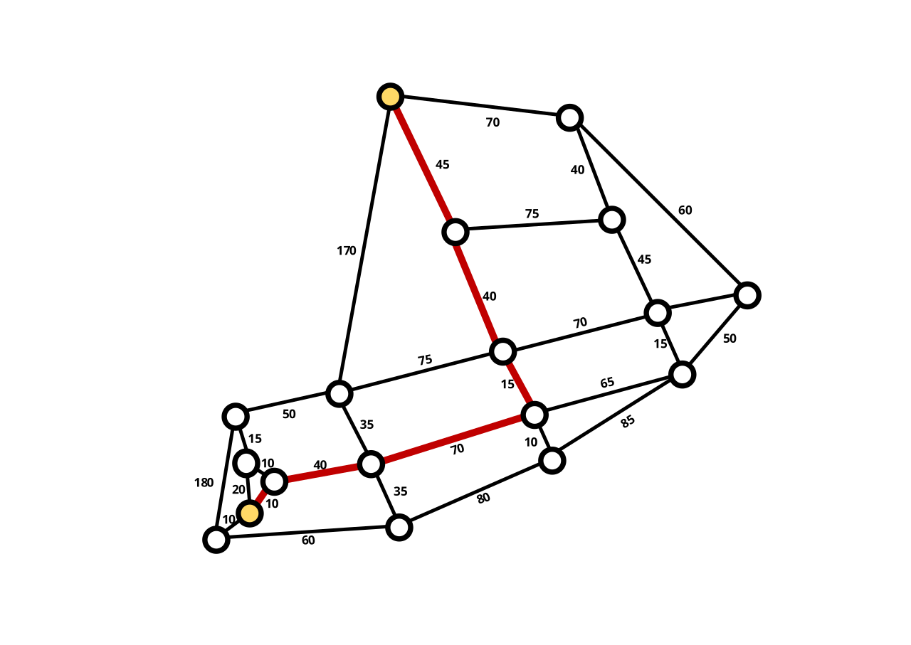
The textbook algorithm for shortest paths is Dijkstra's algorithm, which explores outward from the start in order of distance until it reaches the destination. On a city graph with millions of edges, that exploration touches a large part of the city for every query. A* speeds it up by preferring nodes in the direction of the destination, and Uber's 2015 post on its routing engine measured a city-scale A* query with live traffic at about 120 milliseconds. That sounds fast, but it's far too slow when every request needs dozens of ETAs and the whole platform asks for hundreds of thousands a second.
The standard trick for fast routing is to precompute. Contraction hierarchies rank the nodes by importance and add "shortcut" edges that skip over unimportant nodes, so a query can climb quickly onto major roads and come back down near the destination, answering in milliseconds. The catch is the precomputation: Uber's post notes that building the contracted graph for all the roads of the world takes about 12 hours, which makes folding in live traffic, which changes by the minute, very hard.
How should ETAs be computed?
- Always uses the latest traffic
- Nothing to precompute
- About 120 ms per query: too slow at scale
- Very fast queries
- About 12 hours to rebuild for the world
- Live traffic is hard to apply
- Fast queries with fresh traffic
- Learns what the graph can't see
- Two systems to build and keep consistent
Uber's in-house routing engine, Gurafu, launched in 2015 and divides the graph into a hierarchy of cells, so that small sections can be preprocessed independently and in parallel, aiming for single-digit-millisecond answers at hundreds of thousands of requests a second. On top of it, since 2022, a model called DeepETA predicts the difference between the routing engine's estimate and the real arrival time, learning effects such as pickups at airports or slow drop-offs that a sum of road segments can't know about.
DeepETA is worth a moment, because it's a neat design pattern. The routing engine computes an ETA as a sum of segment travel times. Then a neural network, which Uber says replaced one of the largest gradient-boosted tree ensembles in the world, predicts how wrong that sum will be, given the time of day, the type of request and other features. Learning only the correction keeps the model's job small and lets the routing engine keep doing what it's good at. Uber's ETAs feed fares, pickup estimates, matching and delivery planning, which is why DeepETA is described as its highest-traffic model.
07Surge pricing, per hexagon
7.1Supply and demand on a map
It's raining, a concert has just ended, and two hundred people near the stadium open the app at once. There are thirty drivers nearby. If prices stay normal, most of those people get no car and the drivers stay put. Raising the price in that area does two things at once: some riders decide to wait or walk, and drivers from nearby areas head towards the stadium. That's surge pricing, and it's computed per area.
Uber's 2018 H3 post says it plainly: surge is calculated by measuring supply and demand in hexagons in each city. A later post on Uber's real-time analytics system, Gairos, describes the calculation as querying the number of requests and the number of available drivers for a hexagon, with over a million events a second flowing into that system. This is where hexagons earn their keep: smoothing a surge value across a hexagon and its six equidistant neighbours avoids sharp price cliffs at cell edges, and treats every direction the same.
Uber's 2021 paper on its real-time data infrastructure describes surge's choices directly: the pipeline favours fresh data and availability over consistency, and events that arrive late for their window are dropped. It runs in several regions at once, and if one region fails, the surge calculation fails over to another. A price computed from slightly incomplete counts a few seconds ago is far better than no price at all.
08During the trip: live updates and storage
8.1Pushing updates to phones
While Ravi drives to Sam, Sam's app shows the car moving and the ETA counting down, and Ravi's app shows directions. The simple way to build this is for each app to ask the server every few seconds for updates. Uber did exactly that at first, and by its own account, at one point 80% of the requests to its API gateway were these polling calls, most of them answering "nothing new".
Uber's fix, described in 2020, was a push platform called RAMEN: each app keeps one long-lived connection open, and the server pushes updates down it when something changes, with a heartbeat every four seconds to keep the connection alive and detect failures. It handled over 1.5 million concurrent connections and over 250,000 messages a second. In 2022 Uber moved it to bidirectional gRPC streams, because with the earlier one-way design the server couldn't tell for up to 30 seconds whether a message had arrived.
That's the same decision WhatsApp made in its section 2, for the same reason: when the server knows first that something has changed, it should tell the phone, not wait to be asked.
8.2Where trips are stored
A trip, once accepted, is a record that must never be lost: it's the basis of the fare, the driver's pay, receipts, disputes and safety investigations. In 2014 Uber outgrew a single Postgres database and built Schemaless, a layer on top of many MySQL databases. Its data model was an append-only map from (row ID, column name, version) to an immutable JSON value. A trip's row had columns such as BASE for the trip itself, STATUS, NOTES and FARE ADJUSTMENTS, and every change wrote a new version instead of updating in place. The data was split across 4,096 fixed shards, each a primary MySQL database with two replicas.
That design later evolved into Docstore, which added Raft-based replication within each partition and strict consistency per partition, at a scale of tens of millions of queries a second. And as section 5.3 described, the trip-handling platform itself moved onto Spanner in 2021 for transactions across shards.
09When a data centre fails mid-trip
9.1The phone remembers the trip
Sam is halfway to the airport when the data centre handling Pune goes dark. The trip is in progress, Ravi is driving, and the servers that knew about the trip are unreachable.
Uber's 2016 description of its stack says that each city is assigned to the closest data centre and backed up in another, and that if one data centre fails, trips fail over to another. The interesting part is what makes that possible for trips already in progress. According to write-ups of a 2015 Uber talk, the dispatch system periodically sent each driver's phone an encrypted digest of the trip's state. If the data centre failed, the phone's next request would land in the backup data centre, which wouldn't recognise the trip, ask the phone for its digest, and rebuild the trip's state from it. The phone, which is present for the whole trip anyway, acts as a backup of its own trip.
On the app side, Uber described in 2020 a small state machine in its mobile client with four states, primary, failover, backup and recovery, that decides which network path to use and moves back only after test requests succeed.
10The whole system
10.1Every box, and why it's there
| Component | What it does | Added because |
|---|---|---|
| Location index | Latest position of every driver, by cell, in memory | A table scan can't find nearby drivers fast (§2, §3) |
| Cell system (S2, H3) | Turns positions into cell IDs; neighbour searches | Density varies; neighbours must be found cheaply (§3) |
| Consistent hashing + membership | Splits cells across nodes; survives node loss | Too much traffic for one machine (§4) |
| Dispatch | Collects requests and drivers, solves the assignment | Greedy matching wastes everyone's time (§5) |
| ETA service | Shortest paths on the road graph, corrected by ML | Straight-line distance misleads (§5, §6) |
| Surge pipeline | Supply and demand per hexagon, as a stream | Prices must react to local demand within seconds (§7) |
| Push channel | One long-lived connection per app | Polling was 80% of API traffic (§8) |
| Trip store | Durable, transactional record of every trip | A trip is a promise that can't be lost or doubled (§5.3, §8) |
10.2From top to bottom
| Level | The choice | Data structure or algorithm |
|---|---|---|
| System | Split data by how wrong it can afford to be | In-memory index for locations, streams for surge, transactions for trips |
| Location index | Bucket drivers by cell | Hash map from cell ID to the set of drivers in it |
| Cells | Hexagons for areas, squares where containment matters | H3 64-bit IDs (base cell + 15 three-bit digits); S2 Hilbert-ordered IDs |
| Neighbour search | Widen ring by ring | gridDisk: 3k² + 3k + 1 cells within k steps |
| Sharding | Cells to nodes | Consistent hash ring in a red-black tree; SWIM gossip |
| Matching | Batch for a few seconds | Bipartite assignment (Hungarian algorithm, min-cost flow) |
| ETA | Road graph plus correction | Weighted directed graph; A*, partitioned precomputation; residual neural network |
| Surge | Per hexagon, per window | Windowed counts in a stream processor; hexagon → multiplier map |
| Trips | One state change at a time | Hierarchical state machines; append-only versioned cells; Spanner transactions |
11What goes wrong, and what it cost
11.1Failures this design has to survive
| What happens | What the user sees | What the design does |
|---|---|---|
| A location index node crashes | Nothing, or a car briefly missing from the map | Its cells move to other nodes; drivers' next updates refill them within seconds |
| GPS is wrong between tall buildings | The car jumps across the map | Positions are snapped to roads and smoothed over successive updates |
| Two dispatchers pick the same driver | The driver gets two offers | Driver state changes atomically, so the second assignment fails |
| A driver ignores the offer | The rider waits longer | The offer times out and the rider joins the next batch |
| A sudden crowd in one hexagon | Long waits, no cars | Surge raises prices there and draws drivers in |
| A data centre fails mid-trip | A brief stall | The city fails over; in-progress trips are rebuilt from state the phones carry |
11.2The tradeoffs, in one table
| Decision | Chosen | Given up | Why it was worth it |
|---|---|---|---|
| Where locations live | Memory, sharded by cell | Durability | They're overwritten every 4 s and heal themselves |
| How to cut space | Hexagons (H3) for areas | Exact parent-child containment | Equal neighbours make area statistics fair and smooth |
| Who owns which cells | Consistent hashing + gossip (2015) | Exact agreement at every instant | No central coordinator; only a dead node's cells move |
| Matching | Batch for a few seconds | The fastest possible answer for each rider | Lower total waiting for everyone |
| Closeness | Road-network ETA | Cheap straight-line distance | Rivers, bridges and traffic decide real wait times |
| Surge data | Freshness over consistency | Exact counts | A slightly wrong price now beats a perfect price late |
| Trip state | Consistency over availability (2021) | Some write latency | A driver can't be in two trips; trips are never lost |
12Summary
- The workload is mostly locations: every driver every four seconds, a quarter of a million writes a second for a million drivers, of which only the latest per driver matters.
- A table ordered by distance can't scale: every query would compute the distance to every driver, and an ordinary index can't sort by distance from a moving point.
- Cut the map into cells and keep drivers in per-cell lists, so a search looks at a few cells, not everyone.
- Geohash, quadtrees, S2 and H3 are four ways to cut it: prefix strings, density-adaptive squares, Hilbert-ordered squares, and hexagons with equidistant neighbours.
- An H3 cell is a 64-bit path: a base cell and one of seven children per resolution, so parents, neighbours and compaction are bit operations.
- The location index lives in memory, sharded by cell, and heals itself after a crash because drivers resend their positions.
- Match on road-based ETA, not straight-line distance, using the cheap cell search to narrow millions of drivers to a few dozen candidates.
- Batch requests for a few seconds and solve the assignment problem, so everyone waits less in total.
- ETAs come from a road graph plus a learned correction: fast precomputed routing, with a model that predicts how wrong it will be.
- Surge is computed per hexagon from streams of events, favouring freshness over exactness.
- Sort data by the cost of being wrong: approximate and self-healing for locations and surge, transactional for trips and payments.
13Build this
A dispatch simulator.
- Install the
h3Python package. Simulate 10,000 drivers moving along random straight lines in a city-sized box, each reporting a position every four seconds of simulated time, and keep a dictionary from resolution-8 cell to the set of drivers in it. - For each simulated request, use
grid_diskwith increasing k until at least 10 free drivers are found. Count how many cells and drivers each search touched. - Match greedily, then match in two-second batches using
scipy.optimize.linear_sum_assignment(an implementation of the assignment problem). Compare average and worst rider wait. - Put all the drivers in one part of the box and none elsewhere, and watch the search cost change; then try a coarser and a finer resolution.
- Compute "surge" as requests divided by free drivers per cell, smooth it over each cell's
grid_disk(1), and draw it.
14Interview questions
beginnerWhy can't you find the nearest driver with an ordinary database index?›
An ordinary index sorts rows by a stored value, but the distance from a rider to a driver isn't stored anywhere; it depends on where the rider is, which changes with every request. Without a spatial index, the database has to compute the distance to every driver and sort them. A spatial index, a grid of cells, geohashes, a quadtree, S2 or H3, groups drivers by area so a search only looks at the few cells around the rider.
beginnerWhy does Uber use hexagons?›
Every neighbour of a hexagon shares an edge with it and is the same distance away, while a square has four edge neighbours and four corner neighbours that are further away. When you compute something over an area and its surroundings, like supply and demand for surge pricing, hexagons treat every direction alike and avoid artefacts at corners. The cost is that hexagons can't be split exactly into smaller hexagons, so moving between resolutions is approximate.
intermediateDriver locations arrive 250,000 times a second. Where do you store them, and what happens when a node dies?›
Only each driver's latest position matters, so keep it in memory, partitioned by cell across many nodes, with a consistent hash ring deciding which node owns which cells. Updates are routed to the owner of the driver's current cell. When a node dies, its cells move to other nodes on the ring, and because every driver resends a position within a few seconds, the new owners are repopulated almost immediately without any backup.
intermediateWhy would you delay matching a rider by a few seconds on purpose?›
Matching each rider greedily the moment they request can give an early rider a driver that a later rider needed far more. Collecting the requests and free drivers in an area for a few seconds and solving the assignment for all of them together lowers the total waiting time. In a two-rider example, greedy gives waits of 2 and 9 minutes, and the batched assignment gives 4 and 3. Uber describes doing this to reduce the average wait for everyone.
deepWhich parts of a ride-hailing system should be eventually consistent, and which must be strongly consistent?›
Sort the data by the cost of being wrong. Driver locations are overwritten every few seconds and heal themselves, and surge counts are statistics where a slightly stale value is fine, so both can be in-memory or streaming and prefer availability. Driver assignment and trip state must be exactly right: a driver mustn't be offered to two riders, and an accepted trip mustn't be lost, so those changes need atomic transitions in a transactional store. Uber moved its trip platform from an availability-first design to Spanner transactions in 2021 for exactly this reason.
deepHow do you compute ETAs fast enough for matching at scale?›
Model the road network as a weighted graph and compute shortest paths, but plain Dijkstra or A* is too slow at city scale with hundreds of thousands of requests a second. Precomputation helps: contraction hierarchies add shortcut edges for millisecond queries, but rebuilding them for the world takes hours, which makes live traffic hard, so engines like Uber's Gurafu partition the graph into cells that can be precomputed independently. Then a learned model, like Uber's DeepETA, predicts the residual error of the routing estimate from features such as time of day and pickup type.
15Go deeper
A location index node crashes. What's lost, and how long until it's back?›
The latest positions of the drivers in its cells. Its cells move to other nodes on the hash ring, and since every driver resends a position every few seconds, those nodes have a complete picture again within seconds. Nothing needs restoring from a backup.
Two points 10 metres apart have geohashes with no common prefix. How?›
They're on opposite sides of a cell boundary where the Z-order curve jumps. That's why a geohash search always checks the neighbouring cells as well as the cell matching the prefix.
How many H3 cells does gridDisk(k = 3) return around a cell away from pentagons?›
3k² + 3k + 1 = 27 + 9 + 1 = 37: the centre cell, 6 in the first ring, 12 in the second and 18 in the third.
Why hexagons, how the hierarchy works, and how surge uses them. The h3geo.org documentation has the resolution table and the bit layout.
How Uber's routing engine models the road graph, why contraction hierarchies didn't fit live traffic, and the residual model on top.
Consistent hashing plus SWIM gossip for application-level sharding, with the driver-location service as the motivating example.
Why the trip platform moved from availability-first to Spanner transactions, and how state machines model trips.
Kafka, Flink and the surge pipeline, including which properties it trades away and why.
The dispatch system as it was in 2015: supply and demand services, S2 cells, Ringpop, and failover with state kept on drivers' phones.
16Related chapters
The same push-over-polling decision, and a contrasting system built around delivering messages. Chapter 49.
Consistent hashing and how keys move when nodes join and leave. Chapter 29.
SWIM, suspicion and gossip, the membership half of Ringpop. Chapter 30.
What it takes to make "one driver, one trip" hold under concurrency. Chapter 19.
The event log under the surge pipeline. Chapter 23.