A team at a research lab has spent a year collecting about 15 trillion tokens of text, and now they want to train a language model on it. They've picked a shape for it, the same as Meta's Llama 3 70B: 80 layers, about 70 billion learned numbers, trained on sequences of 8,192 tokens at a time. They've written the training code and tested it on a tiny version of the model on one GPU, where it trains happily. They point it at the full-size model on one H100 and press go.
It dies within seconds with an out-of-memory error. And when someone works out how long the job would take if memory weren't a problem, the answer is about two hundred years of one H100 running flat out. One GPU, in other words, is too small for this model by a factor of roughly sixteen, and too slow for it by a factor of thousands.
So the job has to be spread over thousands of GPUs, connected by links inside each server and a network between servers, all working on one model at once. This chapter follows the team as they build that up, asking one question the whole way: how do you split one training run across thousands of GPUs so that it fits in memory, finishes in weeks, and survives the hardware breaking along the way? We'll count what one training step needs, split the work three ways, match each split to the wires between GPUs, make each GPU's share cheaper, and finish with failures and with how to tell whether the whole machine is doing useful work.
01What one training step needs
1.1A training step in plain words
Chapter 45 described a language model as a big collection of learned numbers called weights (also called parameters), which the model uses to turn text into a prediction of the next token, a short piece of a word. Training is how those weights get their values. It starts from random weights and repeats one small procedure, a training step, hundreds of thousands of times.
One step goes like this. The model takes a batch of text, many sequences of 8,192 tokens each, and runs it through all 80 layers. At every position it predicts the next token. This is the forward pass. Its predictions are compared with the tokens that come next in the text, and the mismatch is boiled down to one number, the loss: how wrong the model was on this batch.
Then comes the expensive part. For every one of the 70 billion weights, the training code works out which direction to nudge it, and by how much, to make the loss a little smaller. That number is the weight's gradient. Gradients are computed by going backwards through the layers, last layer first, in the backward pass. Finally, a piece of code called the optimizer uses the gradients to update the weights, and the step is done.
?Why does the backward pass need the forward pass's results?
Because a layer's gradient depends on what went into it. To work out how a layer's weights should change, the backward pass needs that layer's inputs and intermediate results from the forward pass. So the forward pass has to keep them in memory until the backward pass reaches that layer. These saved intermediate results are called activations, and for a big model they take an enormous amount of memory.
Nearly every large model is trained with an optimizer called Adam. It keeps two running averages for every weight, one of recent gradients and one of their squares, and uses them to pick a sensible step size per weight. That means two extra numbers stored for every weight, for the whole of training.
How much arithmetic is a step? Chapter 45 showed that pushing one token through a model costs about one multiply and one add per weight, 2 FLOPs per weight. The backward pass costs about twice as much, because each layer computes gradients for both its inputs and its weights. So training costs about 6 FLOPs per weight per token, a rule from OpenAI's scaling-laws paper (Kaplan et al., 2020). Meta's Llama 3 paper (July 2024) agrees with it: 6 × 405 billion weights × 15.6 trillion tokens is the 3.8 × 10²⁵ FLOPs it reports for its 405B model.
1.2Counting the bytes
Now we can add up what the team's one GPU has to hold. The script below works out the model's size from its shape (Table 3 of the Llama 3 paper), then counts every kind of memory one step needs.
Memory comes in two kinds. Model states are the weights, their gradients and Adam's numbers, and they're the same size whatever batch you train on. Weights and gradients are stored in BF16, the 2-byte format from chapter 45. Adam's numbers and a master copy of the weights are kept in FP32, the 4-byte format, for reasons section 7 covers. That makes 16 bytes per weight, the figure Microsoft's ZeRO paper (2019) uses for this kind of training. Activations depend on how much text is in flight. For them the script uses the count from NVIDIA's paper on activation memory (Korthikanti et al., 2022): about 34 bytes per token per unit of the model's width, per layer, when the big attention score table isn't stored, as with FlashAttention (a chapter 45 card). Llama's layers are shaped a bit differently, so that line is probably off by some percent either way. Its last lines turn the 6-FLOPs rule into time on one H100 at its 989 dense BF16 teraFLOPS.
# The 70B model's shape (Llama 3 70B, Table 3 of the Llama 3 paper)
layers, h, ffn, heads, kv_heads, vocab = 80, 8192, 28672, 64, 8, 128_000
head_dim = h // heads                                   # 128

attn = h*h + 2 * h*(kv_heads*head_dim) + h*h            # Q, K, V, output
mlp  = 3 * h*ffn                                        # gate, up, down
N = layers * (attn + mlp) + 2 * vocab*h                 # + input and output embeddings
print(f"parameters: {N/1e9:.1f} billion")

GB = 1e9
rows = [("weights, bf16 (2 B)", 2*N), ("gradients, bf16 (2 B)", 2*N),
        ("fp32 master weights (4 B)", 4*N), ("Adam m, fp32 (4 B)", 4*N),
        ("Adam v, fp32 (4 B)", 4*N)]
for name, b in rows:
    print(f"  {name:27s} {b/GB:7,.0f} GB")
states = sum(b for _, b in rows)
print(f"  {'model states (16 B/param)':27s} {states/GB:7,.0f} GB")

s = 8192                                                # tokens in one sequence
act = 34 * s * h * layers                               # bytes, Korthikanti et al. eq. 1 without the 5as/h term
print(f"  {'activations, one sequence':27s} {act/GB:7,.0f} GB")
print(f"total for one sequence: {(states+act)/GB:,.0f} GB = {(states+act)/(80*GB):.0f} H100s' worth of HBM")

tokens = 15e12
flops = 6 * N * tokens
peak = 989e12                                           # H100 SXM dense BF16
year = 365*24*3600
print(f"training compute: {flops:.2e} FLOPs")
print(f"one H100 at 100% of peak: {flops/peak/year:,.0f} years; at 40%: {flops/(0.4*peak)/year:,.0f} years")parameters: 70.5 billion
weights, bf16 (2 B) 141 GB
gradients, bf16 (2 B) 141 GB
fp32 master weights (4 B) 282 GB
Adam m, fp32 (4 B) 282 GB
Adam v, fp32 (4 B) 282 GB
model states (16 B/param) 1,129 GB
activations, one sequence 183 GB
total for one sequence: 1,311 GB = 16 H100s' worth of HBM
training compute: 6.35e+24 FLOPs
one H100 at 100% of peak: 204 years; at 40%: 509 yearsThe shape adds up to 70.5 billion weights, about 2 billion of them in the two tables that turn tokens into vectors and back.
Model states come to 1,129 GB, and look at where they go. Only 141 GB of it is the BF16 weights the model computes with. Three quarters is the optimizer's bookkeeping: the FP32 master copy and Adam's two averages, 846 GB together. Then a single sequence of 8,192 tokens adds about 183 GB of activations, and a real batch has thousands of sequences. Storing the attention score table too would make the activations about ten times larger, so every large training run uses FlashAttention or something like it.
And the last line is the other problem. Even if memory were free, one H100 at its theoretical peak, which no real program reaches, would need two centuries. At 40%, a good real-world figure that section 10 explains, it's five.
1.3Two problems
So the team has two separate problems. Their job is too slow for one GPU by a factor of thousands, and the model is too big for one GPU by a factor of about sixteen, before even counting a realistic batch. An H100 has 80 GB of HBM, and our step needs over 1.3 TB.
Adding GPUs can fix either one, depending on how the work is split. Our first split attacks the slowness: give every GPU a copy of the model and a different part of the batch. Let's see how far that gets, and pretend for a section that the model fits.
02Data parallelism: many copies, one model
2.1Copies of the model, slices of the batch
The team plans a batch of 2,048 sequences of 8,192 tokens each, about 16.8 million tokens per step, the same batch size in tokens that Meta used for most of Llama 3 405B's training (it started at 4 million and doubled twice). Suppose they have 8 GPUs. Give each GPU its own complete copy of the model and 256 of the 2,048 sequences, and let all eight run the forward and backward pass at once.
This is data parallelism: every GPU holds the same model and works on different data. Each GPU is driven by its own process, called a rank, numbered 0 to 7. The ranks never need each other's activations, because each sequence stays on one GPU.
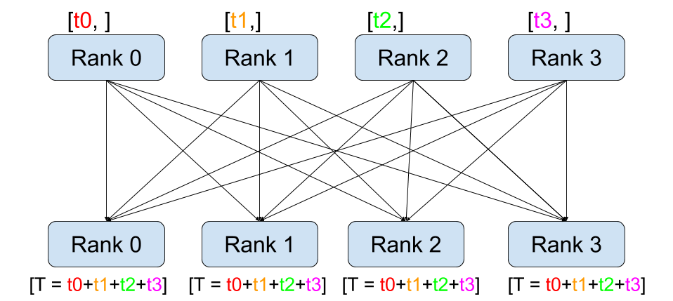
They do need each other at the end of the backward pass. Rank 0's gradients describe how to improve the model on its 256 sequences, and rank 1's on its own 256. For the whole batch, the right gradient is the average of all eight. If each rank updated its weights with only its own gradients, the eight copies would drift apart into eight different models. So before the optimizer runs, every rank needs the sum of all eight ranks' gradients (dividing by eight is done locally). An operation where several ranks combine their data and every rank ends up with the result is called a collective, and this one, summing across all ranks and handing every rank the total, is called an all-reduce.
2.2The obvious way to sum gradients
An obvious design picks one rank to do the adding. Every other rank sends it its full set of gradients, it adds them up, and it sends the total back to everyone. A machine in this role used to be called a parameter server.
Count the bytes. In BF16, the team's gradients are 141 GB. With 8 ranks, the adding rank receives 7 × 141 GB, about 990 GB, through its one network link, and sends as much back out. At 50 GB/s, the speed of one GPU's network card (section 4.2 explains the figure), the receiving alone takes about 20 seconds while seven other links sit nearly idle, and 64 ranks would push 63 copies through that one link. We'd like every link to carry an equal share instead, so that adding GPUs adds links in proportion to the work.
2.3The ring
Here is a scheme with that property. Arrange the ranks in a ring, where each rank sends only to the next one and receives only from the previous one. Cut every rank's gradients into as many equal chunks as there are ranks: with 4 ranks, 4 chunks, called c0 to c3. Then run two phases.
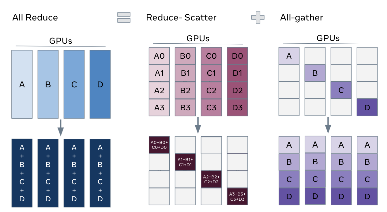
In the first phase, every rank sends one chunk to its neighbour, which adds it to its own copy of that chunk. All ranks do this at the same moment, each on a different chunk, so every link is busy. After 3 rounds (one fewer than the number of ranks), every rank holds one chunk containing the sum from all 4 ranks, a different chunk on each rank. This phase is called a reduce-scatter: the sum gets computed, and it ends up scattered across the ranks, a quarter on each.
In the second phase, the ranks pass those finished chunks around the same ring, each rank copying what arrives. After 3 more rounds every rank has every finished chunk. This phase is called an all-gather. A reduce-scatter followed by an all-gather is an all-reduce.
Now count what each GPU sent: one quarter of its gradients per round, 3 rounds per phase, so 1.5 times its gradients. With N ranks there are N − 1 rounds per phase, each sending 1/N of the data, so each rank sends 2(N − 1)/N times its data. NVIDIA's NCCL documentation derives the same factor.
The team's gradients are 141 GB. With 8 ranks in a ring, each rank sends about 247 GB during the all-reduce. If they grow to 4,096 ranks, how much does each rank send?
We can run a real ring. The script below starts N processes, connects each to the next with a pipe (a one-way channel between processes, provided by the operating system), and gives each a gradient of 960,000 random 4-byte numbers. Each process runs the two phases as in the scene: it sends a chunk to the next rank (from a background thread, so that two neighbours sending large chunks at once can't block each other), receives one from the previous rank, and adds it or keeps it. At the end it checks every rank's result against a plain sum and reports the bytes each rank sent.
import random, threading
from array import array
from multiprocessing import Pipe, Process, Queue

def worker(rank, n, grad, to_next, from_prev, results):
    k = len(grad) // n
    chunks = [grad[i*k:(i+1)*k] for i in range(n)]       # n equal chunks
    sent = 0
    def step(out):                                        # send one chunk to the next rank, receive one from the previous
        nonlocal sent
        t = threading.Thread(target=to_next.send_bytes, args=(chunks[out].tobytes(),)); t.start()
        got = array("f"); got.frombytes(from_prev.recv_bytes()); t.join()
        sent += len(chunks[out]) * 4
        return got
    for s in range(n - 1):                                # reduce-scatter: add what arrives
        got = step((rank - s) % n)
        i = (rank - s - 1) % n
        chunks[i] = array("f", (a + b for a, b in zip(chunks[i], got)))
    for s in range(n - 1):                                # all-gather: keep what arrives
        got = step((rank + 1 - s) % n)
        chunks[(rank - s) % n] = got
    results.put((rank, sent, sum((c.tolist() for c in chunks), [])))

def ring_allreduce(n, size):
    random.seed(n)
    grads = [array("f", (random.randint(-9, 9) for _ in range(size))) for _ in range(n)]
    links = [Pipe() for _ in range(n)]                    # link r carries rank r -> rank r+1
    q = Queue()
    procs = [Process(target=worker, args=(r, n, grads[r], links[r][0], links[(r - 1) % n][1], q))
             for r in range(n)]
    for p in procs: p.start()
    res = sorted(q.get() for _ in range(n))
    for p in procs: p.join()
    want = [sum(g[i] for g in grads) for i in range(size)]
    ok = all(r[2] == want for r in res)
    sent = res[0][1]
    print(f"{n:2d} ranks: all hold the sum: {ok}; each sent {sent/1e6:.2f} MB"
          f" = {sent/(size*4):.3f} x its gradient; 2(n-1)/n = {2*(n-1)/n:.3f}")

if __name__ == "__main__":
    for n in (2, 4, 8, 16):
ring_allreduce(n, 960_000) # 960,000 floats = 3.84 MB per rank 2 ranks: all hold the sum: True; each sent 3.84 MB = 1.000 x its gradient; 2(n-1)/n = 1.000
4 ranks: all hold the sum: True; each sent 5.76 MB = 1.500 x its gradient; 2(n-1)/n = 1.500
8 ranks: all hold the sum: True; each sent 6.72 MB = 1.750 x its gradient; 2(n-1)/n = 1.750
16 ranks: all hold the sum: True; each sent 7.20 MB = 1.875 x its gradient; 2(n-1)/n = 1.875Every rank ends with exactly the sum. (The gradients are small whole numbers, so adding them in a different order can't change the result through rounding.) Now the bytes: going from 2 ranks to 16 multiplies the ranks by eight, and each rank's traffic only goes from 1 times its gradient to 1.875 times, matching the 2(n − 1)/n at the end of each line.
So a large all-reduce takes about 2 × (data size) ÷ (one link's bandwidth), whatever the number of ranks. For the team's 141 GB of gradients that's about 282 GB per rank: about 0.6 seconds if every rank had NVLink's 450 GB/s in each direction, and about 5.6 seconds at a server network link's 50 GB/s.
?If the ring is so good, why does anyone use anything else?
Because each round also waits for a message to cross one link, and a ring of N ranks takes 2(N − 1) rounds one after another. Meta's Llama 3 paper puts the latency across its large training network at up to tens of microseconds. At 4,096 ranks and 10 µs a round, the rounds alone add about 80 ms, a lot for a small message. So NCCL also has tree-shaped algorithms with far fewer rounds, and picks one by message size and rank count.
2.4NCCL, and hiding the all-reduce behind the backward pass
On GPUs, NVIDIA's NCCL (the NVIDIA Collective Communications Library, pronounced "nickel") runs all-reduce, reduce-scatter, all-gather and the other collectives as GPU kernels. When the job starts it finds out how the GPUs are connected, builds rings and trees that follow the fastest links, and then moves data over NVLink inside a server and over the network between servers. PyTorch, JAX and the other frameworks call it underneath. Its benchmark, nccl-tests, reports bus bandwidth: data size divided by time, multiplied by the 2(N − 1)/N factor, so the result can be compared directly with a link's rated speed.
One more trick makes data parallelism cheap. The backward pass finishes the last layer's gradients while the first layers are still being worked on, so there's no reason to wait for the whole backward pass before summing. PyTorch's DistributedDataParallel groups gradients into buckets of a few tens of megabytes and starts an all-reduce on each bucket as soon as it's full, while the GPU carries on with earlier layers. On a fast enough network almost all of the all-reduce hides behind the backward pass.
So data parallelism solves the slowness, in principle: 4,096 GPUs each doing 1/4,096 of the batch, plus an all-reduce that costs about the same at any scale. But we pretended the model fit. Each rank holds a complete copy of the 1,129 GB of model states, and that's 14 times an H100's memory.
03Sharding the copies: ZeRO and FSDP
3.14,096 identical copies
Look at what data parallelism stores. Every one of the team's 4,096 GPUs would hold the same 141 GB of weights, the same 141 GB of gradients and the same 846 GB of master weights and Adam state: about 4.6 petabytes of memory holding one 1.1 TB thing 4,096 times.
Microsoft's ZeRO paper (Rajbhandari et al., 2019; "Zero Redundancy Optimizer") starts from that waste. Each rank keeps only a 1/N slice of the model states, called a shard, and gets the rest from the other ranks at the moment it's needed. ZeRO does this in three stages, each sharding one more kind of model state.
Stage 1 shards the optimizer state. The 846 GB of master weights and Adam averages are touched once per step, by the optimizer at the very end. So make each rank responsible for updating only 1/N of the weights, and give it only their optimizer state. It then needs the summed gradients for just its own slice, which is what the reduce-scatter half of an all-reduce produces. After updating its slice it needs everyone else's updated weights, which is an all-gather. Together that's the same traffic as the all-reduce from section 2. In the paper's words: "4x memory reduction, same communication volume as DP".
Stage 2 shards the gradients as well. Each rank only uses the summed gradients for its own slice, so it can drop the rest once they've been sent on. Same traffic again, and 8 times less memory for model states.
Stage 3 shards the weights themselves. Each rank permanently holds 1/N of the BF16 weights. Just before computing a layer, in the forward pass and again in the backward pass, the ranks all-gather that layer's weights, use them, and free them. Model-state memory is now divided by the number of ranks. The price is the extra all-gather in the backward pass, which brings the traffic to about 3 times the size of the weights instead of 2, "a modest 50% increase in communication volume".
Here is what each stage leaves on one GPU for the team's model, sharded across all 4,096 GPUs:
| What each GPU holds | Plain data parallelism | ZeRO stage 1 | Stage 2 | Stage 3 |
|---|---|---|---|---|
| BF16 weights (141 GB in total) | 141 GB | 141 GB | 141 GB | 0.03 GB |
| BF16 gradients (141 GB) | 141 GB | 141 GB | 0.03 GB | 0.03 GB |
| Master weights and Adam (846 GB) | 846 GB | 0.2 GB | 0.2 GB | 0.2 GB |
| Per GPU | 1,129 GB | 282 GB | 141 GB | 0.28 GB |
| Traffic per step, in units of the weights' size | 2 | 2 | 2 | 3 |
?Why doesn't stage 3 cost far more than 1.5 times?
Because the all-gathers happen one layer at a time, ahead of need. While layer 12 is being computed, the all-gather for layer 13 is already running, so as long as the network keeps up, the GPU never waits for weights. Extra bytes only become extra time when the network can't keep ahead of the arithmetic.
For a 70B model, only stage 3 gets the model states down to something an 80 GB GPU can hold.
3.2FSDP: ZeRO stage 3 in PyTorch
PyTorch's version of stage 3 is called Fully Sharded Data Parallel, or FSDP (Zhao et al., "PyTorch FSDP: Experiences on Scaling Fully Sharded Data Parallel", VLDB 2023). You wrap each transformer layer as one FSDP unit. FSDP then keeps each unit's weights sharded and runs the sequence below for every unit in turn:
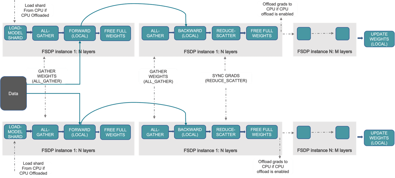
FSDP prefetches the next unit's all-gather while the current unit computes, the overlap from section 2.4 again. It also offers settings that trade memory for traffic. FULL_SHARD is stage 3. SHARD_GRAD_OP keeps the full weights between the forward and backward pass, which saves the backward all-gather at the cost of memory, close to ZeRO stage 2. HYBRID_SHARD shards within one group of GPUs and keeps whole copies across groups, which section 6 will find useful. Meta used a variant of the second idea for Llama 3: its paper says the weights were not resharded after the forward pass, "to avoid an extra all-gather communication during backward passes".
3.3What sharding can't touch
With FSDP across 4,096 GPUs, the model states take 0.28 GB per GPU. It looks solved, until we remember the other line in the TryIt: 183 GB of activations for one sequence.
Sharding doesn't help with those. Under data parallelism every GPU still runs every layer on its own sequences and keeps each layer's activations for the backward pass. Weights can be borrowed one layer at a time, but activations belong to the GPU that computed them, and one sequence's need more than twice an H100's memory.
There's a second limit, which will matter later. Data parallelism splits the batch, and the batch has 2,048 sequences, so beyond 2,048 ranks there's nothing left to split. To go further, and to make one sequence's activations fit, we need to split the work inside the model itself.
04Tensor parallelism: splitting each layer
4.1Splitting one matrix multiply
Look inside one of the 80 layers. Most of its weights and arithmetic sit in the feed-forward block (or MLP), which does two matrix multiplies with a simple function in between. Its first multiply takes each token's 8,192 numbers and widens them to 28,672 using a weight matrix of 8,192 rows and 28,672 columns. (Llama's version, SwiGLU, uses two such matrices side by side and combines them; the splitting works the same way.) An elementwise function is applied to each of the 28,672 numbers on its own. A second multiply narrows them back to 8,192 with a matrix of 28,672 rows and 8,192 columns.
Now cut the first matrix by its columns into 8 slices of 3,584 columns each, one per GPU. Every GPU gets a copy of the input, 8,192 tokens × 8,192 numbers, multiplies it by its slice, and ends up with 3,584 of the 28,672 widened numbers for every token. The elementwise function looks at one number at a time, so each GPU applies it to its own 3,584 without talking to anyone.
Then cut the second matrix by its rows, matching: GPU 0 gets rows 0 to 3,583, the rows that multiply the 3,584 numbers it already has. Each GPU's result is full-size, 8,192 numbers per token, but only a partial sum, because a matrix multiply adds up contributions from every row. Adding the 8 partial results so that every GPU has the total is an all-reduce, now on activations instead of gradients.
This scheme, columns first and rows second so that the only communication is one all-reduce at the end, comes from NVIDIA's Megatron-LM paper (Shoeybi et al., 2019). It's called tensor parallelism, because every weight tensor (the general name for a table of numbers like these matrices) is split across the GPUs. Here it is with 2 GPUs instead of 8:
The layer's other big block, attention, splits the same way. Its 64 attention heads (chapter 45 introduced heads) work independently of each other, so each of 8 GPUs takes 8 query heads, and with Llama 3 70B's 8 shared key/value heads, exactly one key/value head per GPU. The attention block's final matrix is then split by rows, and one all-reduce adds the partial outputs. So a layer needs "only two all-reduces in the forward path and two in the backward path", as the Megatron paper puts it. In 2019 it trained an 8.3-billion-parameter model this way on 512 V100 GPUs at 15.1 petaFLOPS, 76% scaling efficiency against a single GPU.
Tensor parallelism also fixes the activation problem. Each GPU holds only its own slice of the widened numbers and its own heads, so most activations shrink by 8. Steps left whole on every GPU, such as layer normalisation (a small step that rescales each token's numbers), can be split along the sequence instead (Korthikanti et al. call this sequence parallelism), and then the 183 GB per sequence becomes about 23 GB per GPU.
4.2Why tensor parallelism stays inside one server
The price is that all-reduce, four times per layer. Each one sums a tensor the size of one layer's output: 8,192 tokens × 8,192 numbers × 2 bytes, about 134 MB per sequence. Here is what that costs across 8 GPUs, compared with the arithmetic it accompanies:
| One all-reduce, per GPU, ring of 8 | 2 × 7/8 × 134 MB | 235 MB |
| Per layer (2 forward, 2 backward) | 4 × 235 MB | 940 MB |
| Per sequence, 80 layers | 80 × 940 MB | 75 GB |
| Time over NVLink, 450 GB/s each way | 75 GB / 450 GB/s | 0.17 s |
| Time over a 400 Gb/s network link, 50 GB/s | 75 GB / 50 GB/s | 1.5 s |
| Arithmetic per sequence per GPU, at 40% of peak | 6 × 70.5 B × 8,192 / 8 / (0.4 × 989 TFLOPS) | 1.1 s |
| communication as a share of compute: NVLink vs network | 15% vs 137% | |
Over NVLink the all-reduces cost roughly 15% of the compute time. Over a network link they'd take longer than the arithmetic itself. And these all-reduces are hard to hide: the next layer needs the summed output before it can start, so the GPU mostly waits for them.
?Why is NVLink so much faster than the network?
Because of how a GPU server is built. NVIDIA's DGX H100 documentation lists eight H100 GPUs per server, connected through four NVSwitch chips that give each GPU 900 GB/s to the others, 450 GB/s in each direction. To reach other servers, each GPU gets one network card of its own, a ConnectX-7 running InfiniBand at up to 400 Gb/s: 50 GB/s each way. Inside the box a GPU can talk to its neighbours roughly nine times faster than it can talk to anything outside it.
Megatron-LM's 2021 paper (Narayanan et al.) turned this into a rule: "tensor model parallelism should generally be used up to degree g when using g-GPU servers". With 8 GPUs per server, tensor parallelism stops at 8.
4.3The team's first plan
Now the team can write down a plan that fits, TP 8 × FSDP 512 for short. Inside each 8-GPU server, tensor parallelism (TP) splits every layer 8 ways. Across servers, FSDP shards each GPU's slice of the model states over the 512 servers, so that GPU 3 of every server holds 1/512 of the third slice, and data parallelism hands each of the 512 groups 4 of the batch's 2,048 sequences.
| Per GPU, 4,096 GPUs (TP 8 × FSDP 512) | Size |
|---|---|
| Model states: 1,129 GB ÷ 8 ÷ 512 | 0.28 GB |
| One layer's weights, gathered for a moment | about 0.2 GB |
| Activations for one sequence: 183 GB ÷ 8 | about 23 GB |
| Communication per sequence: tensor-parallel all-reduces over NVLink | 75 GB, about 0.17 s |
| Communication per step: FSDP over the network, 3 × (141 GB ÷ 8) | about 53 GB, about 1.1 s, overlapped |
It fits with room to spare, and it's a standard recipe: PyTorch's TorchTitan project, a reference training codebase, ships a Llama 3 70B configuration (on its main branch in October 2026) that sets tensor parallelism to 8 and shards everything else with FSDP. At a realistic 40% of peak, the run would take about 45 days.
Suppose the team wants it done in about 11 days, on 16,384 GPUs. With tensor parallelism stuck at 8, data parallelism would need 2,048 groups of one sequence each, the very last split the batch allows. Or suppose their next model is the 405B one, whose single sequence needs about 72 GB of activations per GPU even after an 8-way split. Either way they need a third way to cut the work, one that doesn't depend on the batch and doesn't need NVLink.
05Pipeline parallelism: splitting by layers
5.1Stages, and the obvious schedule
The model is a stack of 80 layers, and each layer only needs the output of the one before it. So cut the stack: layers 1 to 20 on one server, 21 to 40 on the next, 41 to 60 on a third, 61 to 80 on a fourth. Each piece is a stage. A sequence's activations flow from stage 0 to stage 1 to stage 2 to stage 3 in the forward pass, and its gradients flow back from stage 3 to stage 0 in the backward pass. This is pipeline parallelism.
Communication between stages is light. At each stage boundary, a sequence's activations cross once going forward and once coming back, the same 134 MB as before, and with tensor parallelism inside each stage each GPU sends only its eighth. It's a plain send from one GPU to another, called point-to-point communication, a handful of times per step instead of four times per layer, which the network between servers can easily carry.
The trouble is the schedule. While stage 0 works on the batch, stages 1, 2 and 3 have nothing to do, and once stage 0 hands it on, stage 0 waits until the backward pass comes all the way back. Each stage is busy roughly a quarter of the time, so four servers do the work of one.
5.2Micro-batches and the bubble
Google's GPipe paper (Huang et al., 2018) fixed most of that. Split each pipeline's batch into smaller micro-batches. Stage 0 runs micro-batch 0 and hands it to stage 1, then starts micro-batch 1 while stage 1 works on 0, like an assembly line. Once all the forward passes are through, the backward passes run the other way, and the weights are updated once at the end with all the micro-batches' gradients added together, the same result as one big batch.
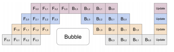
Idle time at the start and the end is called the bubble. With p stages, it's p − 1 forward passes at the start and p − 1 backward passes at the end. Doing the useful work takes m micro-batches' worth of passes, so the bubble is (p − 1)/m of the useful time, the formula in the Megatron-LM 2021 paper. Four stages and 16 micro-batches waste 3/16, about 19%. GPipe found the overhead "negligible when M ≥ 4 × K", their names for the micro-batches and stages.
More micro-batches shrink the bubble, but GPipe's schedule has a memory problem: every micro-batch's forward pass finishes before any backward pass starts, so each stage holds the activations of all m micro-batches at once. So fixing the bubble makes the memory problem worse.
5.3One forward, one backward
The way out is to start backward passes earlier. Microsoft's PipeDream (Narayanan et al., 2018) introduced a schedule called 1F1B, one forward, one backward. Each stage runs just enough forward passes to fill the pipeline, and from then on alternates: one forward pass of a new micro-batch, then one backward pass of the oldest unfinished one. The synchronous version used by Megatron-LM, sometimes called PipeDream-Flush, also stops at the end of every batch to update the weights, like GPipe.
Four stages, eight micro-batches, and a backward pass takes twice as long as a forward pass. Compared with GPipe's schedule, what does 1F1B do to the time per step?
The script below simulates both schedules for 4 stages and 8 micro-batches, with a forward pass taking 1 time unit and a backward pass 2. Each stage works through its list of passes in order, and a pass starts only when its stage is free and the pass it depends on is done (the previous stage's forward pass, or the next stage's backward pass, of the same micro-batch). In the timelines a digit is a forward pass of that micro-batch, a letter is a backward pass (a for micro-batch 0, b for 1, two characters wide because it takes twice as long), and a dot is idle time. "Peak stored" is the most micro-batches whose activations a stage held at once.
P, M = 4, 8              # pipeline stages, micro-batches per step
TF, TB = 1, 2            # a backward pass takes about twice as long as a forward

def gpipe(s):            # every forward, then every backward
    return [("F", i) for i in range(M)] + [("B", i) for i in range(M)]

def one_f_one_b(s):      # a few forwards to fill the pipe, then alternate
    warm = min(P - s - 1, M)
    order = [("F", i) for i in range(warm)]
    f, b = warm, 0
    while b < M:
        if f < M: order.append(("F", f)); f += 1
        order.append(("B", b)); b += 1
    return order

def simulate(schedule):
    done, free = {}, [0] * P
    todo = [schedule(s) for s in range(P)]
    grid = [[] for _ in range(P)]
    live = [0] * P; peak = [0] * P
    while any(todo):
        for s in range(P):
            if not todo[s]: continue
            kind, i = todo[s][0]
            dep = ("F", s - 1, i) if kind == "F" and s > 0 else ("B", s + 1, i) if kind == "B" and s < P - 1 else None
            if dep and dep not in done: continue
            start = max(free[s], done.get(dep, 0))
            end = start + (TF if kind == "F" else TB)
            grid[s] += ["."] * (start - len(grid[s])) + [str(i) if kind == "F" else "abcdefgh"[i]] * (end - start)
            free[s] = done[(kind, s, i)] = end
            live[s] += 1 if kind == "F" else -1
            peak[s] = max(peak[s], live[s])
            todo[s].pop(0)
    total = max(free)
    for s in range(P):
        print(f"  stage {s}: {''.join(grid[s]).ljust(total, '.')}   peak stored: {peak[s]}")
    busy = M * (TF + TB)
    print(f"  step takes {total} units, each stage busy {busy}: idle {1 - busy/total:.0%} of the time")

for name, sch in (("GPipe", gpipe), ("1F1B", one_f_one_b)):
print(name); simulate(sch)GPipe
stage 0: 01234567.........aabbccddeeffgghh peak stored: 8
stage 1: .01234567......aabbccddeeffgghh.. peak stored: 8
stage 2: ..01234567...aabbccddeeffgghh.... peak stored: 8
stage 3: ...01234567aabbccddeeffgghh...... peak stored: 8
step takes 33 units, each stage busy 24: idle 27% of the time
1F1B
stage 0: 0123......aa4bb5cc6dd7ee.ff.gg.hh peak stored: 4
stage 1: .012....aa3bb4cc5dd6ee7ff.gg.hh.. peak stored: 3
stage 2: ..01..aa2bb3cc4dd5ee6ff7gg.hh.... peak stored: 2
stage 3: ...0aa1bb2cc3dd4ee5ff6gg7hh...... peak stored: 1
step takes 33 units, each stage busy 24: idle 27% of the timeIn the GPipe rows, each stage does all eight forward passes, waits (the dots in the middle) for the first backward pass to come down from the stage above, then does all eight backward passes. Every stage is idle for 9 of the 33 units: (p − 1) × (1 + 2) = 9, which is 3/8 of the 24 units of useful work, the (p − 1)/m formula. And every stage held all 8 micro-batches' activations at its peak.
In the 1F1B rows, stage 3 does each forward pass and immediately its backward pass (0aa, then 1bb), never holding more than one micro-batch. Stage 0 runs four forward passes, waits for the first backward pass to come back, and then alternates. The step still takes 33 units and the dots have only moved around. But peak memory is 4 micro-batches on stage 0 and fewer further along, and that cap of p doesn't grow with the number of micro-batches. So with 1F1B the team can use many micro-batches to shrink the bubble without running out of memory.
5.4Interleaving, and the batch-size squeeze
Even the bubble itself can be shrunk. Megatron-LM's 2021 paper proposed giving each GPU several small, separate pieces of the model instead of one big one: with 4 stages and 80 layers, GPU 0 might hold layers 1–4, 21–24, 41–44 and 61–64. Each pass through one piece is shorter, so filling and draining the pipeline takes less time, and the bubble shrinks to (p − 1)/(v · m) for v pieces per GPU. The price is v times as many point-to-point sends. This interleaved schedule is what Meta used for Llama 3, with 16 pipeline stages, and its paper gives the bubble ratio as (PP − 1)/(V × M).
There's a squeeze hidden in that formula. The batch is fixed at 2,048 sequences, because the people training the model choose it for how well the model learns, not for the hardware. Each pipeline gets 2,048 ÷ (number of data-parallel groups) of them as micro-batches. Add GPUs as more data-parallel groups and each pipeline gets fewer micro-batches, m falls, and the bubble grows. Meta saw exactly this: on 16,384 GPUs with 128 data-parallel groups, utilization dropped from 43% to 41% compared with 8,192 GPUs and 64 groups, "due to the lower batch size per DP group needed to keep the global tokens per batch constant".
So the team has three ways to cut the job. Next comes how to combine them on one cluster, and which wires each one should use.
06Putting the three together on a real network
6.1Three axes, one grid of GPUs
Combining all three is called 3D parallelism. Picture the GPUs as a three-dimensional grid. Along one axis, groups of 8 share every layer with tensor parallelism. Along the second, groups of p stages hold consecutive layers as a pipeline. Along the third, d copies of that whole arrangement each take a share of the batch, as data parallelism with FSDP. The number of GPUs is the product, 8 × p × d. PyTorch calls such a grid a device mesh, and its tutorials draw a two-axis version:
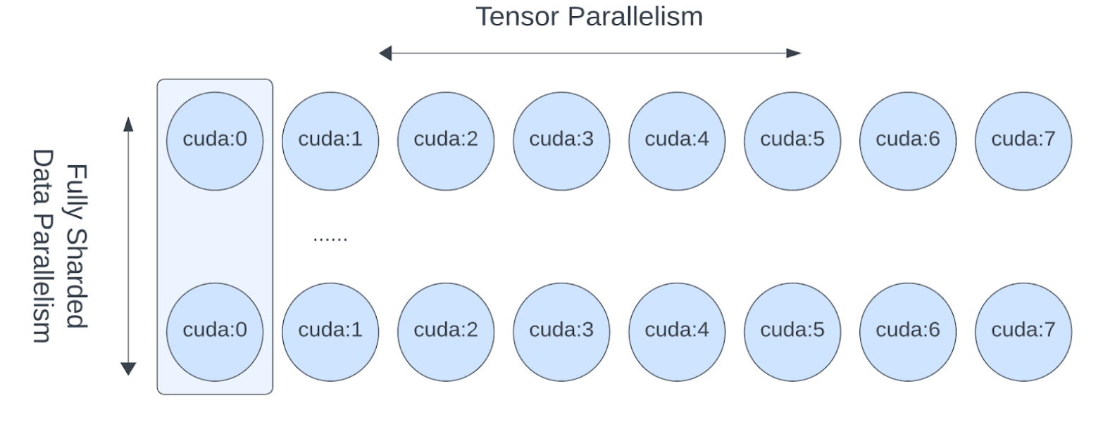
Llama 3 405B added a fourth axis, context parallelism, which splits each very long sequence across GPUs so that training on 131,072-token sequences fits. Table 4 of its paper lists the actual grids:
| GPUs | Tensor | Context | Pipeline | Data (FSDP) | Sequence length | Utilization (BF16 MFU) |
|---|---|---|---|---|---|---|
| 8,192 | 8 | 1 | 16 | 64 | 8,192 | 43% |
| 16,384 | 8 | 1 | 16 | 128 | 8,192 | 41% |
| 16,384 | 8 | 16 | 16 | 8 | 131,072 | 38% |
The order of the axes matters more than the numbers, because each axis creates a different kind of traffic. Put the team's model through each axis and the pattern is plain:
| Axis | What crosses | How often | Can it overlap with compute? | Wants |
|---|---|---|---|---|
| Tensor | All-reduce of one layer's output, about 75 GB per sequence per GPU | 4 per layer | Barely: the next layer waits for it | NVLink |
| Pipeline | One sequence's activations at a stage boundary, 134 MB ÷ 8 per GPU | Twice per micro-batch per boundary | Mostly, with enough micro-batches | Any link |
| Data (FSDP) | All-gathers of weights and a reduce-scatter of gradients, about 53 GB per GPU | Spread through each step | Yes, by prefetching the next layer | Bandwidth; tolerates latency |
Meta's paper states the rule: "The innermost parallelism requires the highest network bandwidth and lowest latency, and hence is usually constrained to within the same server. The outermost parallelism may spread across a multi-hop network and should tolerate higher network latency." Their order, innermost first, was tensor, context, pipeline, data.
6.2The network between servers
Inside a server, as section 4.2 found, NVSwitch connects every GPU to every other at 450 GB/s each way. Between servers it's a network, and it has to carry every pipeline send and every FSDP collective for thousands of GPUs at once.
Large training clusters give every GPU its own network card, which is why a DGX H100 has eight of them. They usually run either InfiniBand, a network built for supercomputers, or Ethernet with RoCE ("RDMA over Converged Ethernet"). Both offer RDMA, remote direct memory access: one machine's network card writes straight into another machine's memory, including GPU memory, without either CPU copying the data. That keeps the CPU and the operating system's network stack (chapter 10) out of the path entirely.

A switch only has so many ports, so thousands of GPUs need switches stacked in layers. Usually the shape is a fat tree (also called a Clos network): servers connect to leaf switches, and every leaf connects to every switch in the layer above. If each leaf has as many cables going up as coming down, any half of the GPUs can send to the other half at full speed. That measure, the bandwidth across the worst way of cutting the cluster in two, is called bisection bandwidth, and a network that provides full bisection bandwidth is called non-blocking.
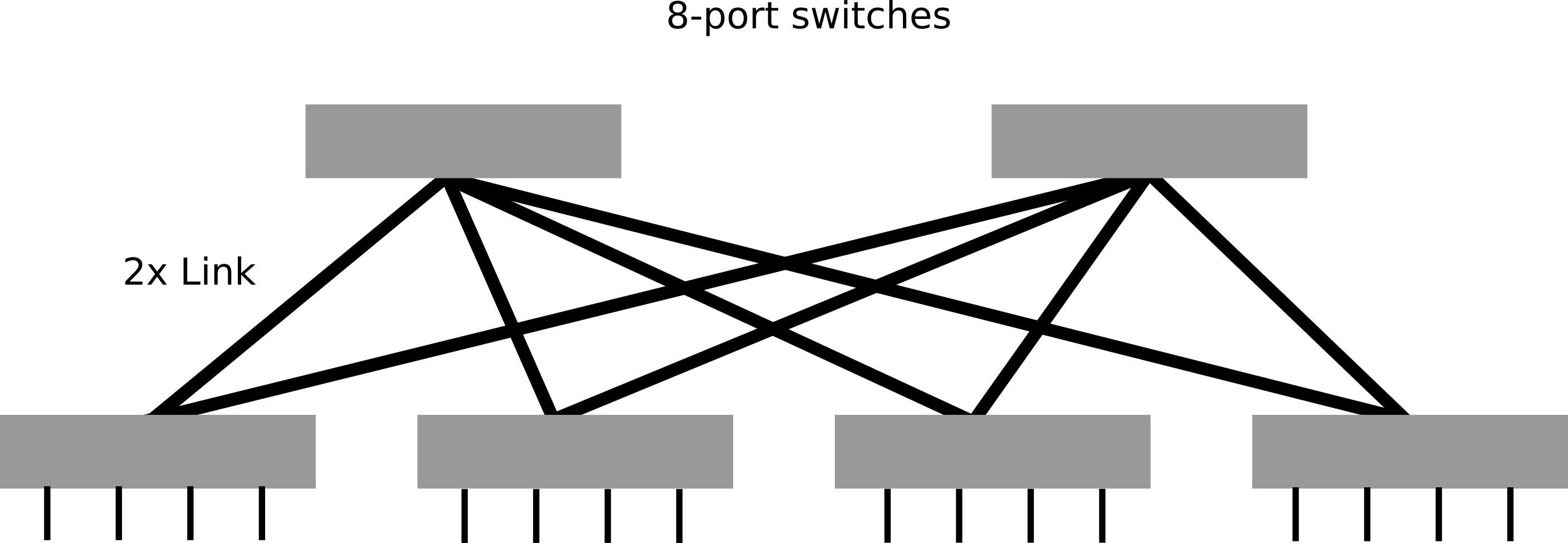
Full bisection bandwidth gets expensive at scale, so real clusters compromise at the top. The Llama 3 paper describes Meta's 24,000-GPU RoCE cluster in three layers. Each rack holds 16 GPUs in two servers under one top-of-rack switch. 192 racks join into a pod of 3,072 GPUs with full bisection bandwidth. Eight pods join into the whole cluster, but at that top layer the network is oversubscribed 1:7, meaning there's one unit of upward capacity for every seven units of demand that could want it. Traffic within a pod is cheap, and traffic between pods is scarce.
So where the grid lands on the cluster matters as much as its shape. Meta's paper says its parallelism layout and job scheduler are "all optimized to be aware of network topology, aiming to minimize network communication across pods". Its collective library also opens 16 network flows between each pair of GPUs instead of one, so the switches can spread the load across more paths. Llama 3 405B ran on RoCE and the smaller Llama 3 models on InfiniBand, both at 400 Gb/s per link and tuned to perform the same.
6.3Placing the team's job
Back to the team's first plan, TP 8 × FSDP 512, on a cluster shaped like Meta's. Each tensor-parallel group is one server, so its constant all-reduces never leave NVLink. The FSDP groups, one per slice, run across all 512 servers, and 512 servers is 4,096 GPUs, more than one 3,072-GPU pod. Every FSDP all-gather would cross the oversubscribed layer.
FSDP's HYBRID_SHARD setting from section 3.2 fits this situation. Shard the model states within each pod and keep a complete sharded copy in each of the two pods. The per-layer all-gathers and reduce-scatters then stay inside a pod, and only one gradient all-reduce per step, between the two copies, crosses the top layer. The memory cost is small: the model states are divided by 2,048 instead of 4,096, about 0.55 GB per GPU instead of 0.28.
Now the plan fits and the wires match the traffic. What's left is making each GPU's own work cheaper: the numbers it stores and multiplies, and the activations it keeps.
07Fewer bits per number: mixed precision
7.1BF16 for the arithmetic, FP32 for the weights
Section 1 said the weights are stored in BF16 and the optimizer's copy in FP32. Now we can see why. A floating-point number is stored in three parts: a sign bit, an exponent that sets how large the number is (its range), and a fraction that holds its significant digits (its precision). FP32 uses 1 + 8 + 23 bits. The older 16-bit format, FP16, uses 1 + 5 + 10, which keeps decent precision but cuts the range so much that its largest value is 65,504. Google's BF16 ("brain floating point") makes the other trade: it keeps FP32's 8-bit exponent, so it covers the same range as FP32, and keeps only 7 bits of fraction, about 2 to 3 decimal digits.
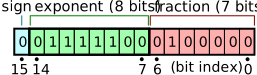
16-bit numbers buy speed and space. Tensor cores multiply BF16 matrices far faster than FP32 ones (chapter 45's H100 figures are 989 dense BF16 TFLOPS against 67 for plain FP32), and half the bytes means half the memory traffic. The script below rounds a few values to each format: Python has FP16 built in (the "e" format of the struct module), and BF16 is made by rounding an FP32 number's bit pattern to its top 16 bits. Then it adds a small training update to a weight of 1.0, once and then a thousand times, in BF16 and in FP32.
import struct

def fp16(x):                       # round to IEEE half precision (5-bit exponent, 10-bit fraction)
    try: return struct.unpack("e", struct.pack("e", x))[0]
    except OverflowError: return float("inf")

def bf16(x):                       # keep fp32's 8-bit exponent, round the fraction to 7 bits
    bits = struct.unpack("I", struct.pack("f", x))[0]
    bits = (bits + 0x7FFF + ((bits >> 16) & 1)) & 0xFFFF0000
    return struct.unpack("f", struct.pack("I", bits))[0]

def fp32(x):
    return struct.unpack("f", struct.pack("f", x))[0]

print("value         fp32            fp16            bf16")
for v in (70000.0, 1e-8, 3.14159265):
    print(f"{v:<13g} {fp32(v):<15.9g} {fp16(v):<15.9g} {bf16(v):.9g}")

w, update = 1.0, 1e-4              # a weight, and one small step of training
print(f"\nweight 1.0 plus an update of 1e-4:")
print(f"  in bf16: {bf16(bf16(w) + bf16(update))}")
print(f"  in fp32: {fp32(fp32(w) + fp32(update)):.9g}")
w16 = w32 = 1.0
for _ in range(1000):
    w16 = bf16(w16 + update); w32 = fp32(w32 + update)
print(f"after 1,000 such updates: bf16 {w16}, fp32 {w32:.6g}")value fp32 fp16 bf16
70000 70000 inf 70144
1e-08 9.99999994e-09 0 1.00117177e-08
3.14159 3.14159274 3.140625 3.140625
weight 1.0 plus an update of 1e-4:
in bf16: 1.0
in fp32: 1.00010002
after 1,000 such updates: bf16 1.0, fp32 1.10002Look at the first three rows: they're the range-versus-precision trade. FP16 can't hold 70,000 at all and turns it into infinity, and it rounds 10⁻⁸ to zero. BF16 holds both, though 70,000 comes back as 70,144 because 7 fraction bits can't do better. Both 16-bit formats round π to 3.140625.
The last lines show why training can't keep its master weights in BF16. Near 1.0, neighbouring BF16 numbers are about 0.008 apart, so adding 0.0001 rounds straight back to 1.0. A thousand updates later the BF16 weight hasn't moved, while the FP32 weight has reached 1.1 as it should. Updates are routinely this small compared with the weights, so a model trained purely in BF16 would partly stop learning.
Training gets around this with the recipe from NVIDIA and Baidu's "Mixed Precision Training" paper (Micikevicius et al., 2017), and the 16 bytes per weight in section 1 pay for it. The forward and backward passes run in 16-bit on the tensor cores. The optimizer keeps an FP32 master copy of every weight and applies updates there, where small updates register, then makes a fresh BF16 copy for the next step. With FP16 the paper also needed loss scaling: multiplying the loss by a large constant before the backward pass so that small gradients don't round to zero (the 10⁻⁸ row), then dividing it back out. BF16's FP32-sized range makes loss scaling unnecessary, the main reason training moved to BF16. Meta went further for sums: Llama 3 accumulates gradients across micro-batches in FP32 and does FSDP's reduce-scatter in FP32 too, after finding numerical problems otherwise.
7.2FP8
Below 16 bits comes 8. A 2022 paper from NVIDIA, Arm and Intel ("FP8 Formats for Deep Learning", Micikevicius et al.) defined two formats: E4M3, with 4 exponent bits and 3 fraction bits, usually used for weights and activations, and E5M2, with 5 and 2, whose extra range suits gradients. Its authors trained language models of up to 175 billion parameters in FP8 and matched the 16-bit results.
The prize is speed: an H100 SXM's datasheet lists 3,958 FP8 TFLOPS with sparsity, which is 1,979 for ordinary dense matrices, twice its BF16 figure. The catch is that 8 bits cover so little range that every tensor needs its own scaling factor, chosen from recent values, to shift its numbers into range. Only the matrix multiplies run in FP8, and the master weights, optimizer and sensitive operations stay in higher precision, so the memory saving is much smaller than the speed-up. Llama 3 was trained in BF16 and uses FP8 only for inference.
Precision shrinks every number, but the biggest flexible item in a GPU's memory is still the activations, about 23 GB per sequence per GPU in the team's plan. One more trick shrinks them: not keeping most of them at all.
08Activation checkpointing: keep less, compute twice
8.1Recomputing instead of storing
The backward pass needs each layer's activations, so the forward pass keeps them. Alternatively, keep only each layer's input, throw away everything computed inside the layer, and when the backward pass reaches it, run the layer's forward pass again from the saved input. This is activation checkpointing, also called activation recomputation. (The word "checkpoint" here means a saved input to restart a computation from. Section 9 uses the same word for saving the whole job to disk, which is a different thing.)
For the team's model a layer's input is 134 MB per sequence, so keeping only the 80 inputs costs about 11 GB per sequence before tensor parallelism, against 183 GB for keeping everything. The price is arithmetic: the forward pass runs twice, and it's 2 of the 6 FLOPs per weight per token, so a step costs roughly 8 FLOPs per weight per token instead of 6, a third more. This idea goes back to Chen et al.'s "Training Deep Nets with Sublinear Memory Cost" (2016), which showed that saving only every √n-th layer's input brings memory down to about √n layers' worth for one extra forward pass.
8.2Recomputing only the cheap parts
A third more arithmetic is a lot to pay. NVIDIA's 2022 paper (Korthikanti et al., "Reducing Activation Recomputation in Large Transformer Models") noticed that activations differ wildly in memory taken per unit of arithmetic needed to rebuild them. The parts of attention that produce the huge score tables take a lot of memory and little arithmetic, and most of the rest is the reverse. Recomputing only the first kind, which they called selective activation recomputation, combined with the sequence parallelism from section 4.1, cut activation memory by 5 times while removing over 90% of the time full recomputation had cost. On a 530-billion-parameter model on 2,240 A100s, utilization went from 42.1% with full recomputation to 54.2%.
Whether the team needs any of this depends on the rest of the plan. Meta's paper says that, after carefully freeing tensors it no longer needed, it "could pre-train Llama 3 on sequences of 8K tokens without activation checkpointing". TorchTitan's 70B recipe turns full activation checkpointing on, which makes room for several sequences per pass, so FSDP doesn't have to all-gather the weights separately for each one. The team would probably measure both. Either way, recomputed arithmetic is work the GPUs do that doesn't train the model, which matters in section 10.
Now the plan is complete, and the team starts the run on 4,096 GPUs, expecting about 45 days. Within hours, a GPU breaks.
09When thousands of GPUs run for weeks
9.1What Meta saw in 54 days
Chapter 45 introduced the best public record of GPU failures at scale, and it comes from this exact situation: section 3.3.4 of the Llama 3 paper, covering 54 days of training the 405B model on up to 16,384 H100s. There were 466 job interruptions: 47 planned (firmware upgrades, configuration changes) and 419 unexpected. About 78% of the unexpected ones were confirmed or suspected hardware problems, and GPU issues alone were 58.7%: faulty GPUs (148), HBM memory (72), on-chip SRAM (19), the GPU's system processor (17), silent data corruption (6) and thermal sensors (6). Network switches and cables caused 35, and software bugs 54.
That's an interruption roughly every 3.1 hours. A single GPU will probably go years without a fault, but sixteen thousand of them together fail several times a day.
?Why does one GPU's failure stop the whole job?
Because every collective in this chapter needs every member. A tensor-parallel all-reduce needs all 8 GPUs of a server, a pipeline stage needs the next stage, and an FSDP all-gather needs every shard. Training is synchronous: nobody starts step 1,001 until everyone has finished step 1,000. One dead GPU leaves 16,383 others waiting inside a collective that will never complete. Meta's paper says it directly: "a single GPU failure may require a restart of the entire job".
9.2Checkpoints, and how often to take them
So the job has to save its state regularly and restart from the last save. A saved copy of the job's state is a checkpoint. It holds everything needed to continue as if nothing happened: the FP32 master weights and Adam's two averages (846 GB for the team's model), the step number, the position in the data so no text is skipped or seen twice, and the random number generators' states. With FSDP each GPU writes its own shard, about 0.2 GB per GPU for the team. Meta's paper quotes 1 MB to 4 GB per GPU for Llama 3, written to a storage system of 7,500 servers delivering 2 TB/s sustained and 7 TB/s at peak, and notes that the "highly bursty checkpoint writes … saturate the storage fabric for short durations".
That scene contains the trade-off. Checkpoint rarely and every failure throws away a lot of work. Checkpoint often and the GPUs spend much of their time paused while they write. A classic rule from Young's 1974 paper on checkpoint intervals puts the best interval at about √(2 × time to save × mean time between failures).
The script below tries it on the team's job. It assumes an interruption every 12 hours on average (a quarter of Meta's rate for a quarter of the GPUs, assuming failures scale with GPU count), 30 seconds of pause per checkpoint, and 10 minutes to detect a failure, swap the server and reload. It simulates the 45-day job at several intervals, with failures at random times, and reports the effective training time: useful training as a share of the time that passed, the figure Meta used for Llama 3's reliability. Each interval is averaged over 20 runs.
import math, random

WORK    = 45 * 24 * 3600   # seconds of useful training the job needs
MTBF    = 12 * 3600        # one interruption every 12 hours on average
SAVE    = 30               # seconds the GPUs pause to take a checkpoint
RESTART = 10 * 60          # seconds to detect, swap the node, reload, warm up

def run(interval, seed):
    rng = random.Random(seed)
    done = wall = 0.0
    next_fail = rng.expovariate(1 / MTBF)
    while done < WORK:
        chunk = min(interval, WORK - done)           # train until the next checkpoint
        if wall + chunk + SAVE <= next_fail:
            wall += chunk + SAVE; done += chunk       # reached the checkpoint safely
        else:
            wall = next_fail + RESTART                # crash: everything since the last checkpoint is lost
            next_fail = wall + rng.expovariate(1 / MTBF)
    return WORK / wall

print(f"Young's rule of thumb: checkpoint every {math.sqrt(2 * SAVE * MTBF) / 60:.0f} min")
for minutes in (2, 10, 27, 60, 180, 600):
    eff = sum(run(minutes * 60, s) for s in range(20)) / 20
print(f"checkpoint every {minutes:3d} min: effective training time {eff:.1%}")Young's rule of thumb: checkpoint every 27 min
checkpoint every 2 min: effective training time 78.8%
checkpoint every 10 min: effective training time 93.2%
checkpoint every 27 min: effective training time 95.0%
checkpoint every 60 min: effective training time 93.7%
checkpoint every 180 min: effective training time 86.6%
checkpoint every 600 min: effective training time 63.1%Checkpointing every 2 minutes spends a fifth of the time pausing to save (30 seconds of every 150). Checkpointing every 10 hours loses hours of work per failure, and a third of the run goes to redoing it. Young's 27 minutes lands at the best value, 95%, and the curve is flat near the top: anything from 10 minutes to an hour costs a percent or two, so the formula is a guide.
Two things lift the whole curve. One is a cheaper save: if the GPUs only copy their shard into the server's CPU memory, which takes seconds, and a background process writes it to storage while training continues, the pause shrinks, and so does the best interval. PyTorch's distributed checkpointing library offers this as async_save. The other is a faster restart. Meta's paper lists reducing "job startup and checkpointing time" first among its measures, and reports above 90% effective training time for Llama 3, with only three interruptions in the 54 days needing significant manual work.
9.3Hangs and stragglers
A failure that stops the job is the easy kind. Harder are the ones that don't stop anything.
Inside a server, GPUs reach each other over NVLink with ordinary memory loads and stores issued from inside a kernel. Meta's paper reports that when a GPU or an NVLink connection fails, this often shows up as "stalled load/store operations within CUDA kernels without returning a clear error code", and the job just hangs. That's what the watchdog in the scene is for: PyTorch's NCCL integration runs a thread that times out a collective stuck for too long. To find the rank to blame, PyTorch has a flight recorder, a ring buffer recording every collective each rank started and finished, which Meta used to diagnose hangs at scale.
Worse still is a GPU that keeps working, only slowly, perhaps running hot and lowering its clock, or with a link that came up at half speed. It's called a straggler, and in synchronous training it sets the pace for everyone, since every collective waits for its slowest member. Meta's paper: "Even a single straggler can slow down thousands of other GPUs, often appearing as functioning but slow communications." The paper even saw the weather in its numbers, a 1 to 2% daily swing in throughput as mid-day heat pushed GPUs to lower clock speeds, and power swings of "tens of megawatts" across the data centre when tens of thousands of GPUs started or stopped together, for instance all waiting for a checkpoint.
All of these, the bubbles, the communication, the recomputing, the failures and the stragglers, cost time. What the team needs is a single number that says how much of the hardware's capacity is turning into training.
10Model FLOPs utilization: one number for the whole machine
10.1Counting only the useful arithmetic
Chapter 45 showed that nvidia-smi's "100% utilization" only means a kernel was running. Training needs a stricter measure, and Google's PaLM paper (Chowdhery et al., 2022) defined the one everyone now uses: model FLOPs utilization, or MFU. It is "the ratio of the observed throughput (tokens-per-second) relative to the theoretical maximum throughput of a system operating at peak FLOPs".
In practice: take the tokens trained per second, multiply by the FLOPs the model needs per token (6 per weight, from section 1), and divide by the number of GPUs times each GPU's peak FLOPS. Everything else counts against it: pipeline bubbles, communication the GPU waits for, slow elementwise operations, stragglers, and recomputation. Leaving out recomputed passes is deliberate, since they don't move training forward. Counting them gives a different figure the PaLM paper calls hardware FLOPs utilization, or HFU. PaLM 540B, on 6,144 TPU v4 chips, reached 46.2% MFU and 57.8% HFU.
| Llama 3 405B, 8,192 H100s | 430 TFLOPS per GPU / 989 peak | 43% MFU |
| Megatron-LM 2021, 1T params, 3,072 A100s | 163 TFLOPS per GPU / 312 peak | 52% of peak |
| Korthikanti et al. 2022, 530B, 2,240 A100s | selective recomputation | 54.2% MFU |
| PaLM 540B, 6,144 TPU v4 | paper's figure | 46.2% MFU |
| good large-scale training lands roughly here | 40–55% | |
So at best roughly half of what the GPUs could do turns into training, and a carefully tuned job probably sits around 40%, the figure the team's estimates have used all along.
?Why can't MFU get close to 100%?
Because much of a training step isn't matrix multiplies. Chapter 45's roofline showed that elementwise operations, normalisations and the like do so little arithmetic per byte that they're limited by HBM bandwidth, and the tensor cores sit idle while they run. Add the pipeline bubble, the tensor-parallel all-reduces that can't be hidden, the occasional wait for a straggler, and the scheduling gaps between kernels, and a few percent here and there adds up to half.
10.2The team's number, and Meta's
MFU turns into a schedule directly. Here is the team's run at the 40% they're hoping for:
| Training compute | 6 × 70.5 B × 15 T tokens | 6.35 × 10²⁴ FLOPs |
| Tokens per step | 2,048 × 8,192 | 16.8 M |
| Compute per step | 6 × 70.5 B × 16.8 M | 7.1 × 10¹⁸ FLOPs |
| Time per step, 4,096 GPUs at 40% MFU | 7.1 × 10¹⁸ / (4,096 × 0.4 × 989 TFLOPS) | 4.4 s |
| Steps | 15 T / 16.8 M | ≈ 894,000 |
| Training time, before failures | 894,000 × 4.4 s | ≈ 45 days |
| at 95% effective training time (section 9), the calendar time is about | 47 days | |
Every point of MFU is worth roughly a day of this run. At 30% it would take 60 days, and at 50%, 36.
Meta's Llama 3 model card (April 2024) gives a real figure to compare with: 6.4 million H100 GPU-hours of pre-training for the 70B model on over 15 trillion tokens. Working backwards, 6.35 × 10²⁴ FLOPs over 6.4 million hours at 989 TFLOPS comes to about 28% of peak. But the card doesn't say what those hours include. If they count restarts, lost work, evaluation runs or experiments, the true MFU of the training itself was higher, so treat 28% as a floor. How Meta split the 70B model across its GPUs is unpublished; the paper's Table 4 covers only the 405B.
11What it all costs
11.1The numbers side by side
Here are the numbers this chapter has relied on, in one place:
12Running it
12.1Commands
Each question this chapter raised has a tool that answers it on a running cluster.
# How are the GPUs in this server connected? (section 4.2)
nvidia-smi topo -m                         # NV18 between GPUs = NVLink; also shows which NIC is nearest each GPU
nvidia-smi nvlink --status

# Is the network link up, and at what speed? (section 6.2)
ibstat                                     # InfiniBand port state and rate ("Rate: 400" is 400 Gb/s)

# What bandwidth does an all-reduce reach? (section 2.3) busbw should approach the link speed
./build/all_reduce_perf -b 8M -e 8G -f 2 -g 8                   # nccl-tests, one server
mpirun -np 64 ./build/all_reduce_perf -b 1G -e 8G -f 2 -g 1     # across servers

# Which rings and transports did NCCL choose? (section 2.4)
NCCL_DEBUG=INFO NCCL_DEBUG_SUBSYS=INIT,GRAPH torchrun ... 2>&1 | grep -E "Ring|Tree|via"

# Launch one rank per GPU on every server (sections 2 to 6)
torchrun --nnodes=512 --nproc-per-node=8 --rdzv-backend=c10d --rdzv-endpoint=$HEAD:29500 train.py

# Find the rank behind a hang (section 9.3): keep a record of recent collectives, dump on timeout
TORCH_NCCL_TRACE_BUFFER_SIZE=2000 TORCH_NCCL_DUMP_ON_TIMEOUT=1 torchrun ... train.py
The busbw column from nccl-tests is the most useful single check. Run it on every new server and whenever something feels slow: far below a few hundred GB/s inside one H100 server, or far below 50 GB/s across servers, means some link, port or card isn't doing its share.
12.2Rules that hold up
- Count the bytes before choosing a split. Model states are 16 bytes per weight, activations scale with tokens in flight, and both have to fit with room left over.
- Tensor parallelism stays inside the NVLink domain. Eight-way in an 8-GPU server; over the network its all-reduces cost more than the arithmetic.
- Use the fewest dimensions that fit. TP inside servers and FSDP across them is enough for a 70B model; add pipeline stages when the batch or the model forces you, and then watch the bubble.
- Keep the micro-batch count well above the number of stages. The bubble is (p − 1)/(v · m), and a fixed batch makes m shrink as you add GPUs.
- Keep master weights in FP32. Small updates vanish in BF16.
- Checkpoint at about √(2 × save time × time between failures), and make saves asynchronous so the interval can be short.
- Measure MFU, not nvidia-smi utilization. MFU counts only the model's useful arithmetic.
12.3What you trade for what
| Technique | You get | You pay | When the bill arrives |
|---|---|---|---|
| Data parallelism | Near-linear speed-up with GPUs | A full copy of the model states on every GPU | As soon as the model has more than a few billion weights |
| ZeRO / FSDP stage 3 | Model states divided by the number of ranks | 1.5× the communication, all-gathers every layer | When the network can't keep ahead of the compute |
| Tensor parallelism | Each layer's weights, compute and activations divided by t | Four all-reduces per layer that the GPU waits for | Immediately, if t is larger than one server |
| Pipeline parallelism | Layers split across servers with little traffic | The bubble, (p − 1)/(v · m) | When adding GPUs shrinks the micro-batches per pipeline |
| BF16 / FP8 | Fast tensor-core math (FP8 is 2× BF16), less memory traffic | An FP32 master copy; scaling factors for FP8 | When updates or gradients are too small to represent |
| Activation checkpointing | Activations cut to about one input per layer | About a third more arithmetic | As lower MFU on every step |
| Frequent checkpoints | Little work lost per failure | GPU time paused to save | When the save interval is too short for the save cost |
12.4Symptom, cause, fix
| Symptom | Likely cause | Fix |
|---|---|---|
| Out of memory on the first step | Model states or activations don't fit | Shard with FSDP, raise TP to 8, turn on activation checkpointing |
| Step time much worse after scaling from 1 server to many | Tensor parallelism crossing servers, or FSDP not overlapping | Keep TP within a server; check prefetching; check busbw across servers |
| MFU falls as GPUs are added, batch unchanged | Fewer micro-batches per pipeline, larger bubble | Interleaved stages, fewer pipeline stages, or a larger batch if the model tolerates it |
| Every rank equally slow, no errors | A straggler: one slow GPU or link | Per-rank compute times, flight-recorder collective timings, then drain the server |
| Job hangs with no error | A stalled NVLink load/store or a dead rank | NCCL watchdog timeout, flight-recorder dump, Xids in dmesg (chapter 45) |
| Loss becomes NaN or stops falling in FP16 | Gradients overflowing or rounding to zero | Use BF16, or loss scaling with FP16 |
| Restarts eat hours | Checkpoints too rare, or slow saves and slow startup | Shorter interval with asynchronous saves; faster job startup |
all_reduce_perf across servers far below 50 GB/s per GPU | Link down to a lower speed, congestion, or traffic crossing an oversubscribed layer | ibstat, switch counters, topology-aware placement |
13Summary
- One GPU is too small and too slow for a 70B model. Model states take 16 bytes per weight (1,129 GB), one sequence adds about 183 GB of activations, and the arithmetic would take one H100 two centuries.
- Data parallelism splits the batch and sums gradients with an all-reduce. In a ring each rank sends 2(N − 1)/N times its data, nearly the same at 8 GPUs or 4,096, and the all-reduce hides behind the backward pass.
- ZeRO and FSDP remove the copies. Sharding optimizer state, gradients and weights divides model states by the number of ranks for 1.5 times the communication.
- Tensor parallelism splits every layer. Columns of the first matrix, rows of the second, four all-reduces per layer, so it stays on NVLink inside one server.
- Pipeline parallelism splits the layers across servers. It costs a bubble of (p − 1)/(v · m), and 1F1B caps each stage's stored activations at p micro-batches.
- 3D parallelism puts the chattiest axis on the fastest links. Tensor inside the server at 450 GB/s; pipeline and data across the network at 50 GB/s per GPU, within full-bandwidth pods where possible.
- Mixed precision computes in BF16 and keeps FP32 master weights, because a 0.0001 update to 1.0 vanishes in BF16. FP8 doubles tensor-core speed again with per-tensor scaling.
- Activation checkpointing trades a third more arithmetic for most of the activation memory; selective recomputation keeps most of the saving for little of the cost.
- At 16,000 GPUs something breaks every few hours. Checkpoint intervals, fast restarts, watchdogs and straggler hunting decide how much of the run is useful.
- MFU measures the whole machine. 40–55% is excellent at scale, and each point is about a day of a 45-day run.
14Build this
Train one model three ways on one machine, and watch the communication.
- Write a small transformer (8 layers, width 1,024) and a training loop in PyTorch. Launch it with
torchrun --nproc-per-node=4, on thegloobackend on a CPU orncclon GPUs. - Wrap it in
DistributedDataParallel. Log step time with 1, 2 and 4 ranks, and check the loss curve matches a single process with the same total batch. - Switch to FSDP (
fully_shardon each layer) and compare each rank's peak memory with the table in section 3.1. - Turn on activation checkpointing per layer. Peak memory should drop sharply and the step should be roughly a third slower.
- Make rank 2 call
time.sleep(0.2)before each backward pass. Every rank's step time rises by the same amount; find rank 2 from per-rank timings alone.
15Interview questions
beginnerWhy can't you train a 70B model on one 80 GB GPU, even slowly?›
Because the model states alone don't fit. BF16 weights and gradients plus Adam's FP32 master weights and two running averages come to about 16 bytes per weight, 1,129 GB for 70.5 billion weights, and one 8,192-token sequence adds about 183 GB of activations. All of it has to be present during a step, so running slowly doesn't help. And the 6.35 × 10²⁴ FLOPs would take one H100 about two hundred years at peak.
intermediateExplain ring all-reduce and why its cost doesn't grow with the number of GPUs.›
Each rank cuts its data into N chunks. In a reduce-scatter of N − 1 rounds, every rank sends one chunk to the next, which adds it to its own, until each rank holds one fully summed chunk. In an all-gather of N − 1 more rounds the finished chunks go round until everyone has all of them.
Each rank sends 2(N − 1)/N times its data, which approaches 2 and stops, and every added rank brings its own link, so the time stays about 2 × size ÷ link speed. What grows is the number of rounds, 2(N − 1), each paying the link's latency, so NCCL also uses tree algorithms for small messages and many ranks.
intermediateWhat do the three ZeRO stages shard, and what does each cost?›
Stage 1 shards the optimizer state (FP32 master weights and Adam's averages, 12 of the 16 bytes per weight); stage 2 also shards gradients; stage 3 also shards the weights. Stages 1 and 2 replace the all-reduce with a reduce-scatter plus an all-gather, the same traffic. Stage 3 all-gathers each layer's weights before using it in both the forward and backward pass, so traffic rises to about 1.5 times, but model-state memory is divided by the number of ranks. PyTorch's FSDP with FULL_SHARD is stage 3.
intermediateHow does Megatron-style tensor parallelism split a feed-forward block, and why not split it across servers?›
The first matrix is split by columns, so each GPU computes its own slice of the widened activations and applies the elementwise function locally. The second is split by rows to match, so each GPU produces a full-size partial sum, and one all-reduce adds them. Attention splits by heads the same way: two all-reduces per layer forward, two backward.
For a 70B model that's about 75 GB per sequence per GPU: 0.17 s over NVLink against about 1.1 s of arithmetic, but 1.5 s over a 50 GB/s network link, and the next layer can't start until each all-reduce finishes.
deepWhat is the pipeline bubble, and what does 1F1B change about it?›
With p stages the pipeline has to fill and drain once per step: p − 1 forward passes at the start and p − 1 backward passes at the end when some stages are idle. With m micro-batches that's (p − 1)/m of the useful time, or (p − 1)/(v · m) with v interleaved pieces per GPU.
1F1B leaves the bubble alone (4 stages and 8 micro-batches idle 27% of the time either way) and caps memory: each stage starts backward passes early and holds at most p micro-batches' activations instead of all m, which makes a large m, and so a small bubble, affordable. At scale, a fixed global batch spread over more data-parallel groups leaves fewer micro-batches per pipeline; Llama 3's MFU fell from 43% to 41% going from 8K to 16K GPUs for that reason.
deepA 16,000-GPU job fails every few hours. How do you choose a checkpoint interval, and what else do you do?›
Young's rule puts the interval near √(2 × save time × mean time between failures). Llama 3 405B saw an unexpected interruption about every 3.1 hours, so a 30-second blocking save gives about 14 minutes. The optimum is broad: a simulation at a quarter of that failure rate gives 95% effective training time at 27 minutes and within a percent or two from 10 to 60.
Then cut the save and restart costs: asynchronous checkpointing to host memory, fast job startup, automatic draining of bad servers with spares ready, a collective watchdog for hangs, a flight recorder to find the stuck rank, and per-rank timing to catch stragglers.
16Go deeper
How many bytes per weight do BF16 weights and gradients plus FP32 Adam state take, and how much is that for 70.5B weights?›
16 bytes: 2 for weights, 2 for gradients, and 12 for the FP32 master copy and Adam's two averages. About 1,129 GB.
In a ring all-reduce over N ranks, how much does each rank send?›
2(N − 1)/N times its data: 1.5× at 4 ranks, 1.875× at 16, just under 2× at any large N.
Why is tensor parallelism usually limited to 8 GPUs?›
Its four all-reduces per layer can't be hidden and need NVLink-class bandwidth; an 8-GPU server's NVSwitch gives about nine times the bandwidth of each GPU's network card.
4 stages, 16 micro-batches, no interleaving: what's the bubble?›
(4 − 1)/16, about 19% of the useful time. With 5 interleaved pieces per GPU, about 4%.
What does MFU leave out that HFU counts?›
Recomputed forward passes from activation checkpointing. MFU counts only the model's own 6 FLOPs per weight per token.
The column-then-row split of each transformer layer, with its f and g communication operators, in a few pages. arxiv.org/abs/1909.08053
How tensor, pipeline and data parallelism combine, the bubble formula, the interleaved schedule, and the "takeaways" for choosing degrees. arxiv.org/abs/2104.04473
The memory accounting behind 16 bytes per weight and the three sharding stages with their communication costs. arxiv.org/abs/1910.02054
How ZeRO stage 3 was built into PyTorch: units, prefetching, sharding strategies, and the memory allocator problems along the way. arxiv.org/abs/2304.11277
Micro-batches and the bubble, then 1F1B scheduling. arxiv.org/abs/1811.06965 · arxiv.org/abs/1806.03377
Algorithm bandwidth versus bus bandwidth, and the 2(N − 1)/N derivation for every collective. github.com/NVIDIA/nccl-tests
Where you meet these ideas in the wild:
16K H100s on a 24K-GPU RoCE cluster with 3,072-GPU full-bandwidth pods and 1:7 oversubscription above them; TP 8, PP 16, FSDP; 38–43% BF16 MFU; 419 unexpected interruptions in 54 days and above 90% effective training time. (paper, §3.3)
540B parameters on 6,144 TPU v4 chips across two pods, 46.2% MFU and 57.8% HFU; Appendix B gives the MFU formula. (paper)
5× less activation memory and 90% less recomputation overhead; 54.2% MFU on a 530B model. (paper)
Its Llama 3 70B recipe sets tensor parallelism to 8, shards the rest with FSDP, and checkpoints activations. (github.com/pytorch/torchtitan)
17Related chapters
HBM, tensor cores, the roofline, NVLink, and the full Llama 3 failure table and Xid codes this chapter builds on. Read it
The other half of a model's life: serving it, where tensor and pipeline parallelism reappear for inference. Read it
Failure rates, redundancy and recovery time, the ideas behind checkpoint intervals and effective training time. Read it
The kernel network stack that RDMA bypasses, and why bypassing it matters at 400 Gb/s. Read it