Someone on your team asks how many copies of shop-api to run next quarter. shop-api is an ordinary web service. Each request, one customer's call such as "show my cart", takes a few milliseconds of work, and a load balancer in front passes every arriving request to one of several identical copies of the service, which we'll call instances. At its busiest the service sees 12,000 requests per second (rps), and a load test says one instance can handle 400 of them at the speed you've promised customers. 12,000 divided by 400 is 30, so you say thirty and go home.
That answer goes wrong in four ways. The 400 is only true up to a point: push an instance much past it and the time each request waits grows without limit. The 12,000 is the peak on a good day, and the day to plan for is the one when a whole data center is down. The thirty copies you ask for take minutes to start, while traffic keeps climbing. And the database behind them doesn't multiply when you add copies. Each of these has a rule you can compute, and most of the rules come from one small result about waiting lines that we'll check first.
Two things do the work. Arithmetic from queueing theory, the mathematics of waiting lines that chapter 16 introduced, tells us how many instances we need. An autoscaler, a program that watches the load and changes the number of instances for you, carries the plan out while traffic moves. This chapter follows one question the whole way: how many instances should shop-api run, and how do we keep that number right as traffic changes? We start by counting requests, move to the fleet, the spare capacity and the autoscaler, and finish with the load test that supplies the numbers and the parts of the system that never scale.
01Requests in flight
1.1Counting what's inside the service
Before counting instances, we need a way to count how many requests the service is handling at the same moment. A restaurant owner deciding how many tables to buy faces the same question. Customers arrive at some rate and each stays for some time, and the number seated at any moment is those two multiplied: 40 people an hour who each stay half an hour fill about 20 seats. Nobody needs a simulation, only the rule.
Requests work the same way. Let λ (lambda) be how many requests arrive per second, which in a steady service is also how many finish, its throughput. Let W be how long each one stays in the service from arrival to reply (its latency), and L how many requests are inside at any instant, whether waiting for a turn or being worked on. Then L = λW. This is Little's Law. It's easy to doubt, because real requests arrive in random bursts and take different amounts of time, so we'll check it.
Save the next program as little.py. It simulates one server where requests arrive at random, 0.8 per millisecond on average, and each takes 1 millisecond of work on average, so the server is busy 80% of the time. The expovariate calls draw those random gaps and work times. For every request the program records +1 at its arrival and −1 at its departure. It then walks through those events in time order, adding up how many requests were inside multiplied by how long they were inside, and dividing by the total time gives the average L. The arrival rate and the average time in the system, W, are measured separately, from counts and timestamps.
import random

rng = random.Random(5)
lam, mu, jobs = 0.8, 1.0, 300_000                 # arrivals/ms and service rate/ms (80% busy)
t = 0.0; free = 0.0; events = []; total_time_in_system = 0.0
for _ in range(jobs):
    t += rng.expovariate(lam)
    start = max(t, free); free = start + rng.expovariate(mu)
    events.append((t, +1)); events.append((free, -1)); total_time_in_system += free - t
events.sort()
area = 0.0; n = 0; prev = 0.0
for time_, d in events:
    area += n * (time_ - prev); n += d; prev = time_
horizon = prev
L = area / horizon                                  # average number in the system
lam_obs = jobs / horizon                            # measured arrival rate
W = total_time_in_system / jobs                     # average time in the system
print(f"average requests in the system  L = {L:6.2f}")
print(f"measured arrival rate       lambda = {lam_obs:6.3f} per ms")
print(f"average time in the system      W = {W:6.2f} ms")
print(f"lambda x W = {lam_obs * W:6.2f} (matches L)")average requests in the system L = 3.96
measured arrival rate lambda = 0.799 per ms
average time in the system W = 4.96 ms
lambda x W = 3.96 (matches L)On average 3.96 requests were inside the system. Requests arrived at 0.799 per millisecond and each spent 4.96 ms there, and 0.799 × 4.96 is 3.96, the same number. The three quantities came from three separate calculations, and the equation held. Notice that a request spends 4.96 ms in a system where its actual work takes 1 ms on average. The other 3.96 ms is spent waiting in line, and the chapter keeps returning to that waiting.
1.2What you can do with it
Little's Law needs no assumptions about how requests arrive or how long they take, so given any two of the three quantities you get the third. If you know your traffic and your latency, you know how many requests are in flight at once, and that sets how many requests the service must be able to hold. We'll use that in section 8 to size a database connection pool.
Knowing how many requests are in flight doesn't yet tell us how many instances it takes to hold them without anyone waiting too long. For that we need to say exactly what a capacity plan has to find out.
02What a capacity plan has to answer
2.1Five questions
A fleet size needs five answers, and Little's Law helps directly with only the last of them.
- What can one instance serve while still meeting the latency target, the response time you've promised?
- What's the peak demand over the period the plan has to cover?
- How many instances does that take, including the failures you've decided to survive?
- How fast can capacity be added, and how much spare capacity covers the gap?
- Which dependencies don't scale with the fleet, and what are their limits?
The Google SRE book, written by the engineers who run Google's services, puts the same thing as three mandatory steps: "an accurate organic demand forecast, which extends beyond the lead time required for acquiring capacity", inorganic demand from launches and campaigns, and "regular load testing of the system to correlate raw capacity (servers, disks, and so on) to service capacity" (Introduction).
2.2Three results from chapter 16, and the job of each
Capacity planning uses three results from chapter 16. None of them is re-derived here. This table says what each is for when you're sizing something.
| Result | What it says | Its job in capacity planning |
|---|---|---|
Utilisation curve, W/S = 1/(1 − ρ) | A server's utilisation ρ is the fraction of time it's busy, and the time a request spends in the system, as a multiple of its service time S, explodes as ρ nears 1 | Sets how busy you plan to run an instance: below the point where waiting explodes, never at 100% |
Little's Law, L = λW | Requests in flight equal throughput times latency | Sizes the pools of workers and connections that hold those requests |
| Universal Scalability Law | Contention (workers queueing for a shared resource such as a lock) and crosstalk (workers spending time keeping each other in step) cap how far adding workers helps | Tells you whether adding instances will work at all, and where it stops helping |
Detail behind each, including why the one-server curve is an optimistic bound, is in chapter 16, sections 3 to 5.
?If the theory is settled, why is capacity planning hard?
Because every input is uncertain. You don't know next month's peak, you don't know exactly what one instance can take, and the thing that adds capacity (an autoscaler, a procurement process) is slow and imprecise. Most of capacity planning is deciding how much margin to keep for each of those uncertainties.
Every other answer in the plan is divided or multiplied by the first one, so that's where we begin: what can one instance of shop-api serve?
03Sizing a fleet
3.1One instance: the rate at the knee
First we need a way to say how fast is fast enough. Averages hide the slow requests, so services describe latency by percentiles. The p99 latency is the time that 99 out of every 100 requests beat, which makes it the slow end that users notice. A latency target is the p99 you've decided the service must stay within, usually a figure agreed with the people who depend on it.
The obvious number for one instance is the most requests per second it can finish, which you find by sending it requests as fast as it will take them.
?Why not plan against the maximum?
Because at that maximum the instance is busy almost all the time. Its utilisation is near 1, and the utilisation curve says the queue, and so the latency, grows without limit there. An instance "doing 600 rps" flat out may be doing it with a p99 of several seconds. Planning to that number means planning to be slow at every peak, so the number we need is lower: the rate at which the instance still meets the latency target.
To find it, we measure a curve instead of a point. We send the instance a fixed rate of requests, the offered rate, record the p99, and repeat at higher and higher rates, plotting offered rate on one axis and p99 on the other. At first the p99 barely moves as the rate rises. Then it starts climbing steeply, and the rate where that happens is the knee. The highest rate that is still inside the latency target sits just before it. Section 7 shows how to measure this against a real database, and why you should repeat the measurement.
| Number | Where it comes from | Use it for |
|---|---|---|
| Maximum throughput | Unthrottled load test; the plateau | Nothing, except finding the knee |
| Knee | Rate where p99 starts rising steeply | The upper bound for planning |
| Planning capacity | Knee, minus margin for measurement noise and variance between instances | Fleet arithmetic |
Suppose shop-api's load test finds each instance comfortable up to 400 rps at the latency target. We'll treat 400 as its planning capacity.
3.2Demand: the peak you can't react inside
The other half of the division is demand. Size for the peak you'll see before you can add capacity, and don't size for the average. Most user-facing traffic has a daily cycle, and a fleet sized for the daily mean falls over at the daily peak.
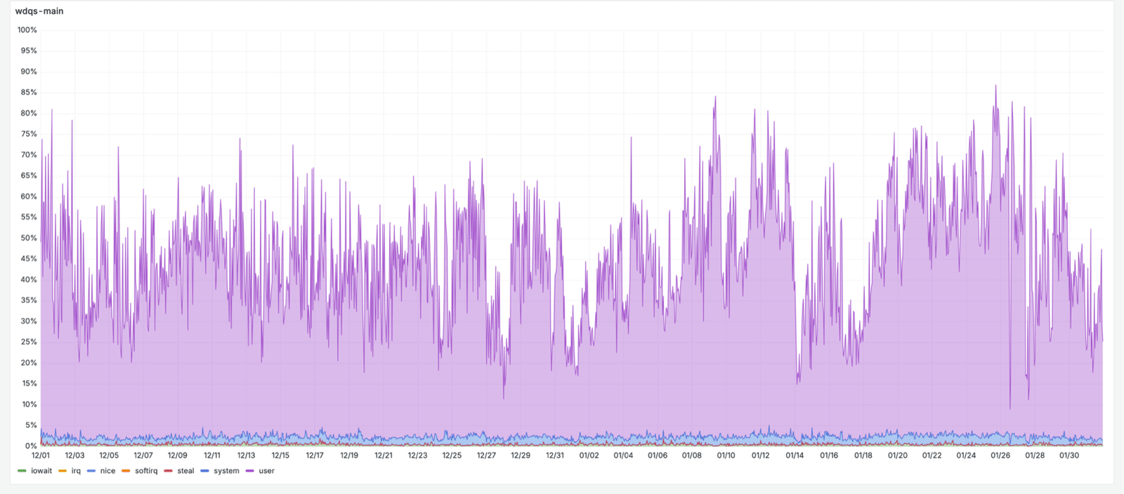
How far ahead the peak has to be forecast depends on the lead time, the time it takes to get new capacity. If adding servers takes two minutes (an autoscaler starting more copies of a program that's ready to run), you plan minutes ahead. If it takes a quarter (buying hardware, raising a cloud quota, provisioning a database), your forecast has to reach past that quarter, which is the SRE book's point above. For shop-api the peak is 12,000 rps.
3.3The arithmetic, with failures included
Now we can divide, and then adjust for what can go wrong. shop-api runs in three availability zones. An availability zone is a separate data center, or group of them, inside a cloud region, with its own power and network, so a fault in one doesn't take down the others. Spreading instances evenly over three zones means we can lose a whole zone and keep running, as long as the instances left can carry the load. Thirty instances cover the peak when everything is healthy. How many do we need if we also want to survive losing one zone at peak?
12,000 rps peak, 400 rps per instance, three zones with equal numbers of instances. How many instances do we need to still carry the whole peak after losing one zone?
The surviving zones are only the first adjustment. A rolling deploy, which replaces instances with the new version a batch at a time, also takes some out of service while it runs, and traffic grows between reviews of the plan. Each line below adds one more thing the fleet has to survive, and the arithmetic compounds.
| Instances for peak, no failures | 12,000 / 400 | 30 |
| Survive losing one of three zones | 30 × 3 / 2 (two zones must carry the peak) | 45 |
| Rolling deploy takes 10% out at a time | 45 / 0.9 | 50 |
| Organic growth before the next review, +15% | 50 × 1.15 | 58 |
| Instances to run, against a naive answer of 30 | 58 | |
The third line allows for 10% of the instances being out during a deploy, so the other 90% must carry the peak. The last line adds growth in traffic before anyone looks at the plan again. At peak, with everything healthy, those 58 instances are each serving about 207 rps, a bit over half of their 400 rps planning capacity. A correctly sized fleet probably looks under-used on a good day, because it's sized for a bad one.
?Why does zone loss cost so much?
Because with three zones, losing one removes a third of capacity, and the other two have to absorb it. Each surviving zone's load rises by half. So the steady-state utilisation you can afford is two-thirds of your per-instance limit. With two zones, it's half. That's the price of zonal redundancy, and it's why many services run in three zones instead of two.
Here's what the zone line in that arithmetic buys, on the 45-instance fleet (15 instances in each zone, before the deploy and growth margins). One detail of the load balancer matters here: it keeps sending each instance a health check, a small regular "are you there?" request, and stops routing traffic to instances that fail several in a row. Watch what each surviving instance has to serve once the balancer has given up on a zone, and compare it with the same failure in a fleet of thirty.
Google's SRE book names a stricter version: N + 2, provisioning "to handle a simultaneous planned and unplanned outage", so peak traffic can be served "while the largest 2 instances are unavailable" (Production Services Best Practices). "Instance" there can mean a whole cluster.
So far we've treated how busy an instance may run as a fixed property of the instance. It also depends on something we haven't looked at: how many servers share the line that requests wait in. That matters for how you divide up a fleet.
3.4Bigger pools run hotter
A pool is a group of servers that take requests from one shared queue. Chapter 16's utilisation curve is for a pool of one. With several servers sharing a queue, a request only waits when all of them are busy at once, which is far rarer, so the picture improves a lot, and capacity planning depends on how much. Take four servers, two of them in each of two separate pools, each pool with its own queue:
The standard result for several servers sharing one queue is the Erlang C formula, which gives the probability that an arriving request has to wait. This table computes it for several pool sizes, where ρ is how busy each server is. Each cell is the probability of waiting, then the mean wait in units of one service time:
| Servers | ρ = 0.5 | ρ = 0.7 | ρ = 0.8 | ρ = 0.9 |
|---|---|---|---|---|
| 1 | 50% · 1.00 | 70% · 2.33 | 80% · 4.00 | 90% · 9.00 |
| 4 | 17% · 0.09 | 43% · 0.36 | 60% · 0.75 | 79% · 1.97 |
| 16 | 1% · 0.00 | 13% · 0.03 | 30% · 0.10 | 59% · 0.37 |
| 64 | 0% · 0.00 | 0% · 0.00 | 6% · 0.00 | 31% · 0.05 |
To read one cell, take the 4-server row at ρ = 0.9, where the servers are busy 90% of the time. 79% of arriving requests have to wait, and the average wait is about two service times. One server at the same utilisation makes a request wait nine.
A pool of 4 servers keeps mean queueing delay under a tenth of a service time up to about 52% utilisation. Merge sixteen such pools into one shared pool of 64 servers. How hot can it run for the same delay?
This shows up anywhere a pool gets split: one thread pool per customer, one queue per partition of the data, one connection pool per pod. Each split trades the efficiency of one large pool for isolation. Sometimes that's the right trade, since isolation stops one noisy customer from starving the others. But it's a trade with a capacity cost you can compute, and it's paid in machines. (Erlang C assumes random arrivals and random service times of the kind the simulation above used, so treat these numbers as the same optimistic bound as the one-server curve.)
Pooling lets a fleet run hotter, but every fleet in this chapter still runs well below what it could carry: the 58 instances of shop-api serve about half their planning capacity on a normal peak. Those idle instances cost money, so someone will ask what they're for.
04What headroom pays for
4.1Five things the gap is for
The gap between what you run at and what you could run at is called headroom. Headroom is the line item finance asks about, so each part of it needs a reason. There are five, and each can be sized.
| Headroom covers | Why it's needed | How to size it |
|---|---|---|
| Bursts | Traffic is burstier than a one-minute average shows | Peak-to-mean at a short interval (per second, not per minute) |
| Failure domains | A zone or a node can vanish | The ×3/2 or N+2 factor from 3.3 |
| Deploys | Rolling deploys take instances out | Divide by the fraction left in service |
| Forecast and measurement error | Next month's peak and per-instance capacity are both estimates | The spread you've seen in both, historically |
| Scaling lag | New capacity arrives minutes after it's needed | Growth rate × time to add capacity (5.5) |
The first three we've already met in the arithmetic. The fourth comes from how loosely we know the inputs, and section 7 shows how loose they can be. The fifth needs a number we don't have yet.
?Why not just run hot and let the autoscaler catch up?
Because the autoscaler is slow compared to the utilisation curve. Near the knee, a few percent more load doubles latency (chapter 16's example: going from 90% to 95% busy takes you from ten service times to twenty). The autoscaler needs minutes to react. For those minutes, headroom is the only capacity you have.
How many minutes? To put a number on the last row of the table, we have to look inside an autoscaler and see where the time goes.
05How autoscalers decide
5.1The Kubernetes loop
Until now the number of instances has been something we choose. In practice the autoscaler from the opening changes it for us as traffic moves, and its delays decide how much headroom we need. We'll look at the one in Kubernetes, the system that most services like shop-api run on.
Kubernetes runs your service as identical copies called pods, each one an instance in our sense. You tell it how many pods you want by writing a number into an object called a Deployment, and that number is the replica count. Kubernetes then starts or stops pods until the running count matches it.
The autoscaler's job is to rewrite the replica count. It works as a feedback loop. It reads a metric, a number the system reports about itself such as the pods' average CPU use, compares it with a target you set, and raises or lowers the replica count to close the gap. Kubernetes' autoscaler is the Horizontal Pod Autoscaler (HPA), "horizontal" because it adds more copies instead of making each copy bigger.
One decision passes through four programs:
- The kubelet runs on each machine in the cluster (Kubernetes calls a machine a node). It starts the pods placed there and measures their CPU use.
- metrics-server collects those measurements from every kubelet.
- The HPA controller is the loop that reads them and decides.
- The Deployment holds the replica count the controller changes.
A new pod doesn't serve traffic the moment it exists. Each pod has a readiness probe, a small check that passes once the service inside can take requests, and only after it passes does the pod count as Ready and receive traffic. Follow one decision from measurement to new pod:
Each pod declares how much CPU it expects to need, its CPU request, and CPU utilisation here means a pod's CPU use as a percentage of that request. The controller's formula is in the HPA documentation. Kubernetes writes CPU in thousandths of a core, so 200m is a fifth of a core. If the pods are using 200m on average against a target of 100m, the ratio is 2 and the replica count doubles; at 50m the ratio is 0.5 and it halves.
Each decision produces a recommendation, the replica count the controller wants at that moment. On a scale-down the HPA doesn't act on the latest recommendation. It remembers the recommendations of the last 300 seconds and takes the highest of them, so one quiet moment can't remove pods that a busy moment will want back. On a scale-up it acts at once, but the pods it orders still have to be placed on a node, have their container image (the packaged program) downloaded, and start. Until each pod is Ready, none of the new capacity exists.
5.2The code that makes the decision
Here's the core of the resource-metric path in the replica calculator:
readyPodCount, unreadyPods, missingPods, ignoredPods := groupPods(podList, metrics, resource, c.cpuInitializationPeriod, c.delayOfInitialReadinessStatus)
removeMetricsForPods(metrics, ignoredPods)
removeMetricsForPods(metrics, unreadyPods)
// ...
usageRatio, utilization, rawUtilization, err := metricsclient.GetResourceUtilizationRatio(metrics, requests, targetUtilization)
// ...
scaleUpWithUnready := len(unreadyPods) > 0 && usageRatio > 1.0
if !scaleUpWithUnready && len(missingPods) == 0 {
	if math.Abs(1.0-usageRatio) <= c.tolerance {
		// return the current replicas if the change would be too small
		return currentReplicas, utilization, rawUtilization, timestamp, nil
	}

	// if we don't have any unready or missing pods, we can calculate the new replica count now
	return int32(math.Ceil(usageRatio * float64(readyPodCount))), utilization, rawUtilization, timestamp, nil
}
// ...
if scaleUpWithUnready {
	// on a scale-up, treat unready pods as using 0% of the resource request
	for podName := range unreadyPods {
		metrics[podName] = metricsclient.PodMetric{Value: 0}
	}
}
Read it from the top. The first three lines sort the pods into ready, not yet ready and missing, and throw away the measurements of pods that are still starting. The usageRatio is current utilisation divided by the target. If every pod is ready and the ratio is within tolerance of 1, the function returns the current count and nothing happens. Otherwise it returns ceil(usageRatio × readyPodCount), which is the formula from 5.1. The last block handles the case we care about: the ratio says to scale up, but some pods are already starting. Those pods are counted as using 0% of what they asked for, which pulls the average down and shrinks the new target.
Two details carry the stability. The tolerance check skips small corrections. And on a scale-up, pods that aren't ready yet are counted as using 0%, so a scale-up already in flight dampens the next one instead of being ignored. Section 6 simulates what happens without that.
?Why ignore the CPU of pods that are starting?
Because starting pods often burn CPU that has nothing to do with load: the Java runtime compiling code as it goes, filling caches, loading classes. According to the docs, the --horizontal-pod-autoscaler-cpu-initialization-period (default 5 minutes) exists to "exclude misleading high CPU usage from initializing Pods (for example: Java apps warming up)". Counting it would make each new pod look overloaded and trigger more scale-up.
5.3The defaults, and what each is for
Each default in the HPA exists to stop one particular misbehaviour:
| Setting | Default | What it prevents |
|---|---|---|
| Sync period | 15 s | Deciding more often than metrics change |
| Tolerance | 0.1 (10%) | Chasing noise around the target |
| Scale-up policy | +100% or +4 pods per 15 s, whichever is more | Unbounded jumps from one bad sample |
| Scale-up stabilisation | 0 s | Nothing: scale-up is meant to be fast |
| Scale-down stabilisation | 300 s (highest recommendation in the window) | Removing pods only to recreate them moments later |
| CPU initialisation period | 5 min | Warm-up CPU triggering scale-up |
| Initial readiness delay | 30 s | Pods flapping Ready/Unready at start |
The docs call the failure these defaults guard against "thrashing, or flapping", a replica count that keeps jumping up and down, and compare the remedy to "hysteresis in cybernetics", where a system reacts to its recent history as well as its current input. Notice the asymmetry in the table: scale-up waits 0 seconds and scale-down waits 300. That's deliberate. Scaling up late costs latency, while scaling down early costs latency and a second scale-up.
5.4AWS target tracking and the cluster autoscaler
Outside Kubernetes, AWS's target tracking policies for EC2 Auto Scaling, which manage groups of virtual machines, work the same way and make the same asymmetric choice. Target tracking "prioritizes availability during periods of fluctuating traffic levels by scaling in more gradually". ("Scaling in" is AWS's term for removing instances, and "scaling out" for adding them.) When a group has several policies, it scales out if any one of them asks, and scales in only if all of them agree. New instances don't count toward the group's metrics until their warmup time has passed, the equivalent of the HPA's readiness handling.
It also says which metrics can't be tracked. The metric "must increase or decrease proportionally to the number of instances". Total RequestCount at the load balancer doesn't change when you add instances; request Latency "doesn't necessarily change proportionally"; a raw queue length has to be divided by the instance count first.
Below the HPA, the Kubernetes cluster autoscaler adds nodes when pods can't be scheduled because the cluster is full, checking every 10 seconds, and removes a node after it has been unneeded for 10 minutes. When a scale-up needs a new node, the node's boot time is added to the pod's.
5.5How long the lag is
Every step above takes time, and the times add up. This is the arithmetic for a morning ramp where shop-api's traffic grows steadily, using rough numbers for a typical HPA setup:
| Traffic growth during the ramp | 2% per minute | |
| Metric window and scrape lag | 60 s average + 15 s | 75 s |
| HPA sync period | up to 15 s | |
| Pod placed, image downloaded, started, Ready | 90 s | |
| Time from need to new capacity | 75 + 15 + 90 | 3 min |
| Traffic growth in that time | 2% × 3 | 6% |
| Headroom above the target just to absorb lag | ≥ 6% | |
The metric is a 60-second average that arrives 15 seconds late, the controller only looks every 15 seconds, and a pod takes 90 seconds to become ready. So by the time new capacity serves traffic, three minutes have passed and the load has grown by 6%. That 6% is the scaling-lag row of the headroom table. If the cluster also has to add a node first, add the node's provisioning time, probably a few minutes more, and lag headroom gets large.
Three minutes of delay is also what makes the autoscaler dangerous. A controller that acts on three-minute-old information keeps ordering capacity it has already ordered, as the next section shows.
06Why autoscalers oscillate
6.1Feedback with delay
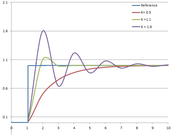
An autoscaler that swings between too few and too many replicas, over and over, is probably one of the most common capacity problems in Kubernetes. It follows from a basic property of feedback loops. A controller that acts on old information will probably overshoot. It sees load that was high a minute ago, adds capacity that arrives a minute and a half from now, and keeps adding in the meantime, since the metric hasn't changed yet. When the capacity lands, it's too much; the controller sees low utilisation and removes it, and the cycle runs again in the other direction.
The delay in an HPA loop has several parts, and they add:
| Source of delay | Typical size | Where it's set |
|---|---|---|
| Metric window | 15–60 s | metrics-server resolution, or the rate window of your monitoring system (Prometheus, for example) |
| Scrape and propagation | 15–30 s | Metrics pipeline |
| Controller period | up to 15 s | --horizontal-pod-autoscaler-sync-period |
| Pod start to Ready | seconds to minutes | Image size, Java start-up, readiness probe |
| New node, if needed | minutes | Cluster autoscaler plus cloud provisioning |
Here is one cycle on shop-api, with the numbers from the lag arithmetic above and no scale-down protection. Each batch of pods is one decision's order. Follow where the batches sit while they start, and what the controller sees in the meantime.
Every part of the loop works as designed, and the delay alone is enough to make it swing. To see how much each safeguard helps, we can simulate it.
6.2A simulation of three policies
The simulation drives a fleet of small pods with one load: 600 rps until t = 300 s, then a step to 1,500 rps, with a 15% sine wave with a four-minute period on top, plus 5% random noise. Each pod serves 100 rps at full CPU, and the target is 60% CPU. The metric is a 60-second average reported 15 s late, pods take 90 s to become ready, and the controller runs every 15 s with the HPA's 10% tolerance. It compares three policies on the same load:
- Policy A compares the number it wants with the pods that are ready, ignoring pods already starting, and scales down at once.
- Policy B counts pods that are still starting, and scales down at once.
- Policy C is B plus the HPA's default 300-second scale-down window.
The core of the loop is below; it steps through the 1,800 seconds one second at a time. The setup around it, not shown, defines base(t) (600 rps, then 1,500 from t = 300), the ready count and the pending list of start-up finish times, recs (the recommendations made so far, with their times) and remove, which takes pods away. Two flags switch between the policies: A sets ignore_pending, and C sets down_window to 300.
for t in range(1800):
    load = base(t) * (1 + 0.15*sin(2*pi*t/240)) * (1 + gauss(0, 0.05))
    while pending and pending[0] <= t: pending.pop(0); ready += 1
    cpu.append(min(1.0, load / (ready*100)))        # saturates at 100%
    if t % 15 == 0 and t > 75:
        m = mean(cpu[t-75:t-15])                     # 60 s window, 15 s late
        ratio = m / 0.6
        cur = ready + len(pending)
        desired = ready if abs(1-ratio) <= 0.1 else ceil(ratio * ready)
        if down_window and desired < cur:            # HPA-style scale-down window
            desired = max(d for (tt, d) in recs if tt > t - down_window)
        have = ready if ignore_pending else cur      # the bug in policy A
        if desired > have: pending += [t+90] * (desired - have)
elif desired < cur: remove(cur - desired)A: ignores pending pods, no window scale-ups 75 scale-downs 30 peak 131 overloaded 1020 s
B: counts pending pods, no window scale-ups 44 scale-downs 32 peak 39 overloaded 760 s
C: counts pending, 300 s down window scale-ups 7 scale-downs 2 peak 35 overloaded 222 s"Overloaded" counts seconds, out of 1,800, when load exceeded 90% of ready capacity. The load needs 21 to 29 pods at the 60% target after the step.
The numbers are medians over eleven random seeds. The last two lines of the output explain the columns: "overloaded" is the number of seconds out of 1,800 when the load was more than 90% of what the Ready pods could handle, and the load itself needs between 21 and 29 pods at the 60% target once the step has happened. So anything much above 29 is waste, and a lot of overloaded seconds is a user-visible problem. Here is one run's replica count over time:
Look at the B line against the "needed" line. B keeps rising when the need is falling and falling when the need is rising. C goes up once, to 35, and stays near the top of the need.
6.3Reading the three policies
Policy A repeats a bug that's easy to write in a home-grown scaler: it compares the desired count with ready pods only, so every 15 s during the 90 s start-up it orders the same pods again. Across eleven seeds its median peak was 131 replicas for a load that needs 29, and it spent 1,020 of the 1,800 seconds overloaded anyway. The HPA avoids this by counting unready and missing pods in its calculation (5.2).
Policy B counts pending pods but scales down immediately. It never ran away, but it chased the four-minute wave with about 75 seconds of metric lag and 90 seconds of start-up, and so it kept arriving at the wrong phase: adding pods as the wave fell and removing them as it rose. It was overloaded for 760 of 1,800 seconds.
Policy C is B plus the HPA's default 300-second scale-down window. It overshot once, to 35, held there, and settled at 29, which covers the peaks of the wave. It scaled 9 times in thirty minutes instead of 76.
?Why was even policy C overloaded for 222 seconds?
Because of the step at t = 300. Utilisation is capped at 100%, so an overloaded fleet reports at most 100 / 60 = 1.67 times the target, and each decision can only grow the fleet by roughly that factor. From 16 pods, it took about 150 seconds to reach the 29 the new load needed. That's scaling lag, and only headroom covers it.
There's a general lesson in B's behaviour. If load has a cycle with a period comparable to your loop's total delay, a fast-reacting autoscaler will chase it out of phase. Either make the loop much faster than the cycle, or make it much slower (a long scale-down window) and provision for the cycle's peak.
6.4Other ways to build an oscillator
Delay isn't the only cause. These are the other ways an autoscaler ends up fighting itself:
| Cause | What happens | Fix |
|---|---|---|
| Scaling on latency | Latency isn't proportional to replicas; near the knee it jumps, far below it barely moves | Scale on a utilisation or per-instance throughput metric |
| Scaling on a raw queue length | Adding consumers doesn't change the backlog proportionally | Divide by consumer count (backlog per pod) and target that |
| Warm-up CPU counted | New pods look overloaded, triggering more scale-up | CPU initialisation period; readiness only when warm |
| HPA and VPA on the same metric | The Vertical Pod Autoscaler (VPA) resizes each pod's CPU and memory requests, so two controllers correct the same error in different ways | The VPA docs say it "should not be used with" the HPA "on the same resource metric (CPU or memory)" |
| Scale-down drains caches | Removed pods take their warm caches; misses raise load on the rest | Longer scale-down windows; shared caches |
| Retries from overload | Overloaded pods time out; clients retry; load rises faster than capacity | Retry budgets and backoff (chapter 40) |
All of this, from the zone arithmetic to the simulation, started from one number we took on trust: that an instance can serve 400 rps at the latency target. It's time to see where that number comes from and how easily it goes wrong.
07Measuring what one instance can take
7.1Open-loop, at fixed rates, stepping up
Getting the per-instance number wrong in either direction costs money or outages, so the test that produces it has to behave like real traffic. The easy way to write a load tester is a loop: send a request, wait for the reply, send the next. That's called a closed loop, and it has a flaw. When the server slows down, the tester slows down with it, so the queue never builds and the test never sees the waiting that real users would. Real customers don't wait for each other before clicking. Chapter 16 explains in detail why a closed loop under-reports exactly the latency you're testing for.
A capacity test sends requests at a fixed rate, on a schedule that doesn't depend on the replies, which is called an open loop. It measures each request's latency from the time it was scheduled to go out, so time spent stuck behind a slow request counts. And it steps the rate up, run after run, until p99 crosses the target, which traces out the curve from 3.1.
For Postgres, the tool is pgbench. It runs a standard set of transactions, small groups of queries the database executes as one unit, and reports transactions per second (tps) and latency. Its --rate option (-R for short) turns it into an open-loop tester. Its docs say the latency it reports "is calculated from the scheduled start times, so it includes the time each transaction had to wait for the previous transaction to finish", and that start times follow "a Poisson-distributed schedule", meaning random gaps of the kind little.py drew with expovariate (pgbench).
# 16 clients on 4 threads, 30 seconds, offered rate $RATE tps, per-transaction log kept
pgbench -c 16 -j 4 -T 30 -R $RATE --log mydb7.2A capacity curve for Postgres
Here's a real one, from a deliberately noisy setup. A Postgres 16 server was pinned to a single CPU with taskset, with fsync=off (so commits don't wait for the disk) and a small 64 MB buffer cache (shared_buffers=64MB), and it served a range query that sums 10,000 rows. pgbench ran sixteen clients on four threads (-c 16 -j 4) on separate CPUs, and the whole setup lived in a 4-CPU container on a virtual machine shared with other workloads. Each repetition first measured the maximum throughput for 10 seconds, then ran 30 seconds at each fraction of that maximum, and p99 was computed from pgbench's per-transaction logs.
| Offered load, % of the capacity just measured | Run 1 p99 | Run 2 p99 | Run 3 p99 |
|---|---|---|---|
| Measured capacity (10 s, unthrottled) | 833 tps | 750 tps | 1,035 tps |
| 30% | 21 ms | 24 ms | 8.6 ms |
| 50% | 56 ms | 133 ms | 190 ms |
| 70% | 411 ms | 80 ms | 8.5 ms |
| 80% | 4.3 s | 2.8 s | 16 ms |
| 90% | 7.3 s | 674 ms | 3.5 s |
| 95% | 703 ms | 59 ms | 11.1 s |
| 105% | 3.6 s | 30 ms | 11.1 s |
Run 3 comes closest to the textbook curve: p99 is under 20 ms at 30%, 70% and 80% of capacity (with one 190 ms blip at 50%), then climbs to seconds at 90% and above, where the backlog grew for the whole 30 seconds. Runs 1 and 2 don't follow it. In run 2, 105% of "capacity" had a p99 of 30 ms, and in run 1, 80% had a p99 of 4.3 seconds.
?Why did the same fraction behave so differently between runs?
Because the capacity itself moved. Ten back-to-back 10-second measurements of the same server, taken straight after these runs, gave 478, 609, 574, 796, 777, 579, 609, 596, 543 and 951 transactions a second. Earlier on the same server, three measurements gave 1,240 to 1,476. Other tenants on the shared VM were taking CPU time, so one core of "Postgres capacity" was a different amount of CPU from minute to minute.
A cloud instance is a milder version of the same thing: noisy neighbours, throttling, different hardware generations behind the same instance type. So per-instance capacity is a range of values with a typical middle and a bad low end, a distribution. Measure it several times, on several instances, and plan to the low end of what you saw. The gap between the median and the low end is the "measurement error" line in the headroom table in section 4.1.
7.3What a capacity test has to include
A step test finds the knee, but a capacity plan leans on more than the knee. This table lists the tests that find the other things, and the thing people tend to skip in each:
| Test | What it finds | What people skip |
|---|---|---|
| Step load | The knee: highest rate inside the latency target | Repeating it, and on more than one instance |
| Soak (hours at planning load) | Memory leaks, garbage-collector growth, compaction, log rotation, cache churn | Running long enough for the slow problems to appear |
| Production-shaped traffic | Real mix of endpoints, payload sizes, cache hit ratios | Replaying or shadowing real traffic instead of one endpoint |
| Dependency limits | The database, cache or third-party API that saturates first | Testing with real dependencies, not mocks |
| Autoscaler ramp | Whether scaling keeps up with a realistic ramp | Ramping at the real rate, from the real minimum |
| Failure at load | What happens when an instance or zone is removed at peak | Killing things during the test, not before it |
That table's fourth row has the most surprising consequences, because the autoscaler we've just studied multiplies the load on whatever it can't scale.
08The parts that don't autoscale
8.1What to check before trusting an autoscaler
An autoscaler adds copies of the stateless tier, the part of the system that keeps no data of its own and so can be copied freely. Everything that tier depends on has fixed capacity until someone changes it, and scaling out moves load onto those things faster.
| Dependency | Its limit | What scale-out does to it |
|---|---|---|
| Database | Connections, CPU, disk operations per second (IOPS) on one primary | More pods, more connections and queries (8.2) |
| Caches | Memory, network bandwidth per node | New pods start cold; misses go to the database |
| Cloud quotas | Instances, IPs, load balancer targets per account | Scale-up fails at the quota, often at peak |
| Downstream APIs | Their rate limits | More callers, more rate-limit errors (HTTP 429), more retries |
| Cluster capacity | Free nodes, IPs in the subnet | Pending pods wait for the cluster autoscaler |
?Why do the dependencies fail at the worst moment?
Because the autoscaler does its most scaling exactly at peak. A fleet that normally runs 10 pods and scales to 40 has never had 40 pods' worth of connections open until the busiest minute of the year. So set maxReplicas, the autoscaler's upper limit on replica count, from what the dependencies can take at that size.
8.2Little's Law for the connection pool
The clearest case is the database connection pool. A connection pool is a fixed set of open connections to a database that a program reuses, so that it doesn't open a new connection for every query. Every pod has its own pool, and the fleet autoscales. For this example take a smaller service than shop-api, one that scales up to 40 pods at peak, with a pool of 10 connections per pod (a common default).
Postgres has a limit of its own. Each connection costs it a process and some memory, so it refuses connections beyond a setting called max_connections, which is 100 by default. The animation follows what happens at peak, and then adds the usual fix, a connection pooler: a small separate program, such as pgbouncer or Amazon's RDS Proxy, that accepts many client connections and shares a few real database connections among them.
The numbers in that animation come from this arithmetic:
| Pods at peak | 40 | |
| Connection pool per pod (a common default) | 10 | |
| Connections the fleet can open | 40 × 10 | 400 |
| Postgres max_connections default | 100 | |
| Concurrent queries needed | L = λW = 2,000 queries/s × 5 ms | 10 |
| Connections the fleet can demand, against what the work needs | 400 vs 10 | |
Little's Law says the database only ever has about ten queries in flight. The fleet is still able to open 400 connections, four times Postgres's default max_connections of 100. Scale-out that works for the app servers breaks the database at the moment traffic peaks.
We now have every piece: the per-instance rate, the arithmetic for the fleet, the headroom, the autoscaler and the limits behind it. What remains is to turn them into something you can review on a Monday morning.
09Reviewing a capacity plan
9.1A checklist for Monday
Each question below comes from one section of the chapter. A plan that can answer all six is a plan someone can check.
- Per-instance capacity (section 7): when was the knee last measured, with what traffic mix, and how many repetitions?
- Peak demand (3.2): what's the forecast peak over the lead time for adding capacity? Include launches.
- Failures sized for (3.3): which zone, instance or deploy failures does the fleet survive at peak? Show the arithmetic.
- Autoscaler (sections 5 and 6): what's the metric, is it proportional to replicas, and what's the total delay from need to Ready?
- Headroom (4.1): which of the five items does it cover, and how much of each?
- Dependencies (section 8): at
maxReplicas, how many connections, requests and IPs does the fleet demand from each dependency?
9.2Looking at it on a real cluster
Each question has a command that answers it on a running Kubernetes cluster with a Postgres database behind it.
# What does the autoscaler see and decide? (section 5)
kubectl get hpa shop-api --watch
kubectl describe hpa shop-api            # current vs target metric, recent scaling events

# How busy is each pod right now, and are any stuck starting? (sections 3 and 5.5)
kubectl top pods
kubectl get pods --field-selector=status.phase=Pending

# Is the database close to its connection limit? (section 8)
psql -c "SHOW max_connections;"
psql -c "SELECT count(*) FROM pg_stat_activity;"
kubectl describe hpa is the most useful of these. It prints the current metric against the target and a list of recent scaling events with their reasons, so a swinging replica count shows up as a sequence of scale-ups and scale-downs a few minutes apart, which you can then compare against the delay table in 6.1.
9.3Rules that hold up
- Plan to the knee, minus a margin. The rate where p99 is still inside the target is the per-instance capacity, measured more than once.
- Put the failures you've chosen to survive into the arithmetic, with their numbers.
- Scale on a metric that moves in proportion to replicas: utilisation or throughput per instance.
- Keep a scale-down window, and provision for the peak of any cycle in your load.
- Test with real dependencies, and set
maxReplicasfrom their limits.
9.4What you trade for what
| You get | You pay | When the bill arrives |
|---|---|---|
| Surviving a zone failure | About 1.5 times the instances for three zones | Every day, as idle capacity on a good day |
| Bigger shared pools that run hotter | Less isolation between customers or data partitions | When one noisy tenant slows everyone |
| Headroom for scaling lag | Extra instances, running all the time | On the cloud bill |
| A long scale-down window | Pods that stay a few minutes longer than needed | Also on the cloud bill, but it buys stability |
| A shared connection pooler | One more component to run and size | When the pooler itself is undersized |
9.5Symptom, cause, fix
| Symptom | Likely cause | Fix |
|---|---|---|
| Replica count swings up and down every few minutes | Loop delay comparable to a load cycle; no scale-down window | Longer scale-down stabilisation; faster start-up; provision for the cycle's peak |
| Scale-up overshoots massively | Controller ignores pods already starting | Count pending pods (HPA does); fix home-grown scalers |
| Latency spikes every morning, then recovers | Scaling lag on the ramp | Headroom for lag (5.5), scheduled pre-scaling |
| New pods trigger more scale-up | Warm-up CPU counted | CPU initialisation period; readiness after warm-up |
| Database falls over during scale-out | Per-pod pools multiplied by replicas | Shared pooler; maxReplicas from the database's limit |
| Fleet fine until a zone fails, then collapses | Sized without the failure factor | Size for ×3/2 (three zones) or N+2 |
| Load test said 600 rps, production struggles at 350 | Test mix, mocked dependencies, or a single noisy run | Production-shaped traffic, real dependencies, repeated runs |
| Autoscaler never scales on a queue metric | Metric not proportional to consumers | Target backlog per consumer |
10Summary
- Little's Law,
L = λW, links requests in flight to arrival rate and latency. In the simulation, 0.799 per ms × 4.96 ms gave the measured 3.96. - Plan to the knee. The rate at which p99 is still inside the target is the per-instance capacity, and the maximum is only useful for finding the knee.
- Put failures in the arithmetic. Surviving one zone of three means running at two-thirds of the limit: 30 instances becomes 45, and 58 with deploys and growth.
- A well-sized fleet looks idle on a good day, because it's sized for a bad one.
- Bigger pools run hotter. For the same queueing delay, 4 servers can run at 52% and 64 at 93%, so every split of a pool costs capacity.
- Headroom pays for bursts, failures, deploys, error and lag, and each part can be sized. Lag alone was 6% in the morning-ramp example.
- The HPA is a delayed feedback loop: 15 s decisions, 10% tolerance, a 300 s scale-down window, and unready pods counted as idle on scale-up.
- Delay makes loops oscillate. In the simulation, ignoring pending pods peaked at 131 replicas for a need of 29, and a scale-down window cut 76 scaling actions to 9.
- Scale on metrics proportional to replicas. Use utilisation or throughput per instance, and leave latency and raw queue length to alerts.
- Measure capacity open-loop, repeatedly, with real dependencies. On a shared machine the knee moved between runs minutes apart.
- Little's Law sizes the pool that matters. 40 pods with 10 connections each can demand 400 from a database whose work needs 10.
11Build this
A capacity model for one service.
- Run a step-load test against one instance with an open-loop tool (
wrk2 -R,oha,k6with an arrival-rate executor, or pgbench-Rfor a database). Repeat it three times and plot p99 against rate with all three runs visible. - Write the section 3.3 arithmetic as a spreadsheet or script with your real peak, zones, deploy strategy and growth, and compare its answer to what you run today.
- Reproduce the simulation in section 6.2, then add a node-provisioning delay and a cache that goes cold on scale-down, and find the scale-down window that keeps replicas stable.
- For each dependency, compute what the fleet demands at
maxReplicas, and lowermaxReplicasor add a pooler where it exceeds the limit.
12Interview questions
beginnerHow do you decide how many instances a service needs?›
Measure what one instance can serve at the latency target (the knee of its p99-against-rate curve, not its maximum), take the forecast peak over the lead time for adding capacity, and divide. Then multiply for the failures you intend to survive, deploys and growth. With three zones, surviving one at peak alone multiplies the count by 1.5.
beginnerWhy does a correctly sized fleet look under-utilised?›
Because it's sized for its worst hour: peak traffic with a zone down during a deploy. In the example in this chapter, a fleet sized that way serves about half its planning capacity per instance on a normal peak. Running it hotter means the bad hour arrives with no room left.
intermediateWalk me through how the Kubernetes HPA decides to scale.›
Every 15 seconds it reads the metric, averages it over ready pods, and computes desired = ceil(current × currentMetric / targetMetric). It does nothing if the ratio is within 10% of 1. Scale-up happens at once, up to doubling or four pods per 15 s; scale-down uses the highest recommendation of the last five minutes. Pods that aren't ready are counted as using 0% on a scale-up, which stops it re-ordering pods already starting.
intermediateYour autoscaler oscillates between 10 and 40 pods. What do you look at?›
Total loop delay first (metric window, scrape lag, sync period, pod start-up, node provisioning) compared with the period of the oscillation and of the load itself. Then whether the metric is proportional to replicas, whether warm-up CPU is being counted, whether a home-grown scaler ignores pending pods, and whether another controller (VPA on the same metric) is fighting it. A longer scale-down window is the usual first fix.
intermediateWhy is scaling on latency a bad idea?›
Latency isn't proportional to replica count. Well below the knee it barely moves as load changes, so the controller gets no signal; near the knee it climbs steeply, so the controller gets a huge one, late. AWS's target-tracking docs list load balancer latency as a metric that doesn't work for the same reason. Scale on utilisation or throughput per instance, and alert on latency.
deepWhy can a large shared pool run at higher utilisation than several small ones?›
Pooling. With c servers sharing one queue, a burst on one is absorbed by idle time on another. Erlang C gives the numbers: for mean queueing delay at or below 0.1 service times, one server can run at 9%, four at 52%, sixteen at 80% and sixty-four at 93%. Splitting a pool per tenant or per shard buys isolation and pays for it in capacity, and that cost can be computed before you pay it.
deepThe app tier autoscales fine but the database falls over at peak. Why, and what do you change?›
Each pod has its own connection pool, so connections scale with replicas even though the database's useful concurrency doesn't. Little's Law gives the real need: queries per second times query time, often tens of connections, while 40 pods with pools of 10 can open 400 against a default max_connections of 100. Put a shared pooler in front, size it with L = λW plus margin, and cap maxReplicas from the database's limits.
13Go deeper
Three zones, 30 instances needed at peak. How many to survive one zone failing at peak?›
- Two zones must carry the whole peak, so each needs half again as much: 30 × 3 / 2.
Which metric can't AWS target tracking use: CPU utilisation, ALB RequestCountPerTarget, or ALB RequestCount?›
RequestCount, the total at the load balancer. It doesn't change when you add instances. Per-target request count does.
What does the HPA assume about pods that aren't ready yet during a scale-up?›
That they're using 0% of the resource request. It dampens the next scale-up and stops the controller ordering the same pods twice.
Why does pgbench -R report latency from the scheduled start time?›
So a transaction that had to wait behind a slow one is charged for the wait. Measuring from the actual start would hide queueing, the thing a capacity test is looking for.
The formula, readiness handling, tolerance, stabilisation windows and default policies. kubernetes.io.
The code quoted in 5.2: grouping pods, tolerance, and zero-usage handling for unready pods. Source.
Warmup, conservative scale-in, and which metrics can't be tracked. AWS docs.
Scan interval, scale-down timing, and what blocks node removal. GitHub.
The three mandatory steps of capacity planning, and N + 2. Introduction · Best practices.
Rate-limited runs, schedule lag, and latency measured from the intended start. Docs.
The Universal Scalability Law applied to real capacity questions, with fitting methods.
14Related chapters
The theory this chapter applies: the utilisation curve, Little's Law, the USL and coordinated omission. Chapter 16.
USE and RED for finding the saturated resource, and CPU throttling in containers. Chapter 41.
Load shedding, retry budgets and the overload behaviour that capacity headroom buys time for. Chapter 40.
cgroups, the mechanism behind pod CPU requests and limits. Chapter 11.