Your checkout service handles about a thousand orders a second, and its dashboard shows an average response time of 40 milliseconds. Everything is green. Then a customer writes in: they pressed "Place order", watched a spinner for almost four seconds, and gave up. Somewhere in that morning's traffic is their request, POST /api/v1/orders, and nothing on the dashboard knows it exists.
The dashboard isn't lying. An average answers the question "how long does a request take, typically?", and a single number can't also say that a few requests took a hundred times longer than the rest. To find this customer's request we needed to write something down about it while it ran. Writing things down costs storage, CPU and money, and at a thousand requests a second the bill grows quickly, so how much to write, in what shape, and how to search it later are real design decisions.
The practice of recording enough about a running system to answer questions about it afterwards is called observability. This chapter asks one question: when one request goes wrong in the middle of a thousand per second, what must we have recorded to find it, and what does that recording cost? We'll start by watching an average hide a slow tail, try the obvious fix of logging every request and price it, count requests instead with a monitoring server called Prometheus, learn how that server stores and searches its numbers and why labels are the bill, then get latency percentiles back out of the counts, and finally follow the one slow request across services with a trace.
01What an average hides
1.1One mean and three percentiles
Let's build a stand-in for the checkout traffic and see what the dashboard's number does with it. The script below makes up 10,000 request times, or latencies (the time from a request arriving to its response going out). Ninety-nine percent of them are around 20 milliseconds, and the other 1% are slow, between 1.5 and 2.5 seconds. It then summarises them four ways: the mean (the average), the median, the p99 and the p99.9.
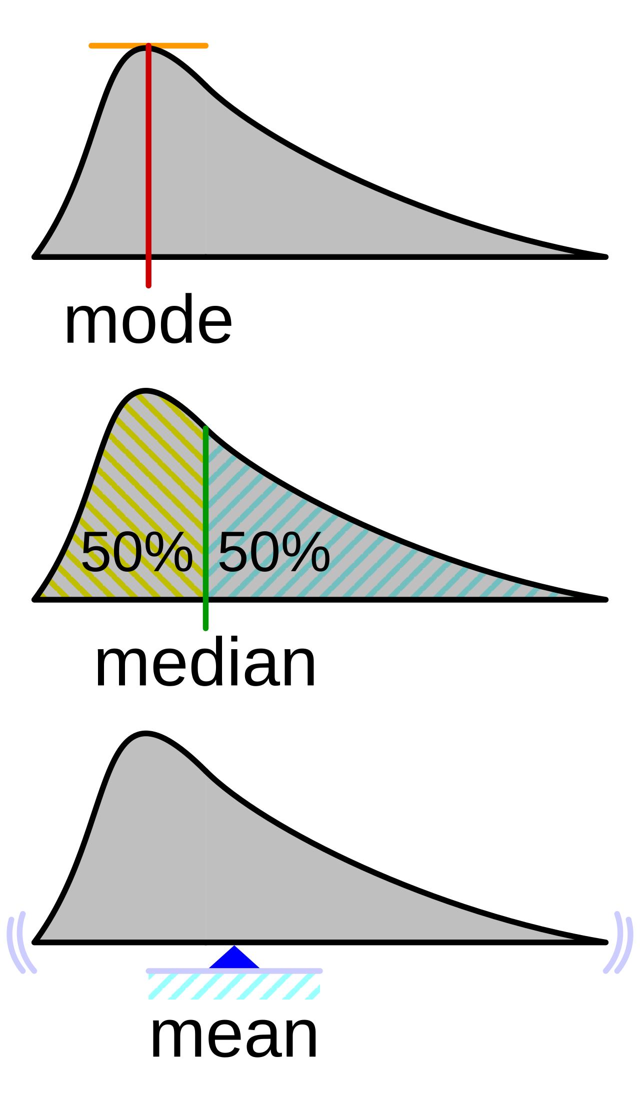
The last three are percentiles. Sort all the requests from fastest to slowest and walk along the list. The median, also written p50, is the request halfway along, so half of the requests are faster than it. The p99 is the request 99% of the way along, so only one request in a hundred is slower. The p99.9 is 99.9% of the way along, with one request in a thousand slower.
In this data 99% of requests take about 20 ms and 1% take about 2,000 ms. Roughly what will the mean be?
The random generator starts from a fixed seed, so you'll get exactly the numbers below when you run it.
import random, statistics

rng = random.Random(11)
lat = [rng.gauss(20, 3) if rng.random() < 0.99 else rng.uniform(1500, 2500) for _ in range(10_000)]   # ms
lat.sort()
print(f"requests : {len(lat):,}   (99% take about 20 ms, 1% take 1.5-2.5 s)")
print(f"mean     : {statistics.mean(lat):7.1f} ms")
print(f"median   : {lat[len(lat) // 2]:7.1f} ms")
print(f"p99      : {lat[int(0.99 * len(lat))]:7.1f} ms")
print(f"p99.9 : {lat[int(0.999 * len(lat))]:7.1f} ms")requests : 10,000 (99% take about 20 ms, 1% take 1.5-2.5 s)
mean : 40.3 ms
median : 20.1 ms
p99 : 1546.2 ms
p99.9 : 2408.3 msCompare the mean with your prediction. The median, 20.1 ms, describes the typical request accurately. The mean, 40.3 ms, is double that and matches nobody's experience, and it's the number our dashboard was showing. The p99 of 1,546 ms sits right at the start of the slow group, because the slow group is exactly 1% of the requests, and the p99.9 of 2,408 ms is deep inside it. Those two describe the requests that made users leave. A hospital that reports its average patient temperature has the same problem: the average can be normal while one patient in a hundred has a dangerous fever.
1.2What we would have to record
Our script could report all of this because it had the full list of 10,000 times in memory. A real service doesn't keep that list, and the dashboard only ever sees whatever summary someone decided to compute. To find our customer's request we need two different things. First, the overall shape of the latencies, kept cheaply and continuously, so that a slow 1% shows up at all. Second, the detail of individual requests, so that when we find a slow one we can see what happened to it.
The simplest way to get both is also the first thing most people try: at the end of every request, write down a line describing it. Let's do that and see what it costs.
02Writing down every request
2.1One structured line per request
A line that a service writes to describe an event is called a log. The easiest log line to write is a sentence, such as order 4412 ok, and the hardest to use: to find slow orders in a pile of sentences you end up searching with regular expressions at 3 a.m. So instead we write one JSON object per event, with the same field names every time. JSON is text with named fields, which every language can read and write, and a log written this way is called a structured log. Here is the line for our customer's request (it's wrapped across lines here so it fits the page; in the log it's one line):
{"ts":"2026-09-27T09:41:07.118Z","level":"info","msg":"request done",
 "service":"checkout","route":"/api/v1/orders","method":"POST","status":201,
 "duration_ms":3712,"trace_id":"4bf92f3577b34da6a3ce929d0e0e4736",
 "span_id":"00f067aa0ba902b7","customer_id":"c_81723"}
Every field answers a question we'll want to ask later. route, method and status say what kind of request it was and how it ended, duration_ms says how long it took (3,712 ms, the almost four seconds our customer waited), and customer_id says whose it was. The two IDs, trace_id and span_id, are there to join this line to other records. The trace ID is a unique name for this request that the services handling it pass along to each other, and section 7 explains how. For now, treat it as a label that will let us find the same request in other places.
With this line written for every request, the complaint is answerable. Search the last hour of logs for customer_id equal to c_81723, and the request is there, with its duration, status and IDs.
2.2What it costs
That line is 262 bytes when written on one line. A thousand requests a second, all day, comes to this:
| One structured log line per request | the JSON line above, on one line | 262 B |
| Requests per day | 1,000/s × 86,400 s | 86.4 M |
| Logs per day | 262 B × 86.4 M | 22.6 GB |
| to write down every request of one service | 22.6 GB/day | |
Nearly all of those 22.6 GB describe fast, healthy requests that nobody will ever look at. And there's a second cost in reading them back. Asking "what fraction of requests in the last hour were slower than a second?" means scanning 3.6 million lines. Logs answer "what happened to this request?" well, and answer "how are we doing overall?" expensively. Two questions follow: how do log systems find a line without reading everything, and how do we keep the volume down?
2.3Searching logs: two ways to index
To avoid reading every line, a log store builds an index, a lookup table made ahead of time so a search can jump straight to the matches. How the store indexes decides both what you can ask it and what it costs:
| Design | Indexes | Fast at | Costs |
|---|---|---|---|
| Full-text (Elasticsearch, OpenSearch) | Every word in every line, in an inverted index | Arbitrary text search across everything | Index size and ingest CPU grow with every word written |
| Label-only (Grafana Loki) | A few tags per stream of lines, such as service="checkout"; the lines themselves stored compressed | Queries that first pick streams by tag, then scan their text | Reads every line of every stream it picked |
An inverted index works like the index at the back of a book. For each word it keeps the list of lines that contain it, so finding every line containing c_81723 means reading one list instead of the whole log. The price is that every word of every line has to be added to some list as it arrives. Loki makes the opposite trade. It groups lines into streams, one per combination of a few tags such as the service name, and indexes only the tags. Its overview says it "does not index the contents of the logs, but only indexes metadata about your logs as a set of labels for each log stream." Writing is cheap, and a query that can't narrow itself down by those tags has to read a lot of text. Loki calls the tags labels, and they follow the same rules as the metric labels in section 5, where you'll see why.
2.4Keeping the volume down
The other lever is writing fewer lines. Each technique below gives up some detail to save storage, and each has a way to go wrong:
| Technique | What it does | Watch out for |
|---|---|---|
| Levels | Keep info and above in production | A debug switch you can flip at runtime is worth more than always-on debug |
| Sampling | Keep 1 in N successful requests, all errors | Sample by trace ID so the logs and trace for a request are kept together |
| Rate limiting | Cap identical messages per second | A loop logging one error a million times still needs to show up once |
| Short retention | Days for raw logs, longer for aggregates | Audit logs have legal retention; keep them separate |
One more hazard comes from writing the line itself. A log call on the request path formats the text, takes a lock on the output, and writes it. At high request rates that synchronous write becomes the latency, and a slow disk, or a full pipe to the log shipper (the agent that carries log lines from the machine to the log store), blocks every request thread until it drains.
Even with all of these, a log is still one record per event, so its cost rises with traffic. What we want for the question "how are we doing overall?" is something whose cost doesn't depend on traffic at all. Counting does that.
03Counting instead of recording
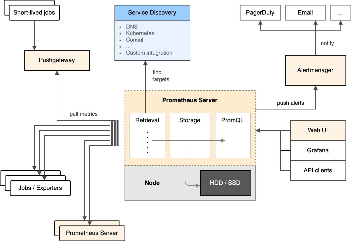
A counter that holds "orders handled so far" takes the same space when the service handles ten requests a second as when it handles a million. The number goes up, and nothing else grows. A number that a service keeps about itself like this is called a metric, and the most widely used system for collecting and storing them is Prometheus, an open-source monitoring server. Its design has been copied by nearly everything since, including most hosted monitoring services, which is why this chapter spends the most time on it.
3.1A series is a name plus labels
One counter for all requests isn't much use, because we'd want to know about failures separately from successes. So the service keeps one counter for each kind of request, told apart by labels: pairs such as method="POST" and status="201" attached to the metric name. Each distinct combination of a name and its labels, together with its history, is called a time series. A single reading on it, a timestamp and a number, is a sample. Here are three series of one metric, each with its first two samples:
http_requests_total{method="POST", route="/api/v1/orders", status="201"} → 1027 @ t1, 1051 @ t2, …
http_requests_total{method="POST", route="/api/v1/orders", status="500"} → 3 @ t1, 3 @ t2, …
http_requests_total{method="GET",  route="/api/v1/orders", status="200"} → 88 @ t1, 90 @ t2, …
Inside Prometheus the name is just one more label, called __name__. A series is its full label set, sorted, and a sample is a (timestamp, float64) pair on it. Our customer's request is one of the increments of the first series.
The metric types, of which there are four, exist only in the client library that the service uses. On the wire and in the database they are all series of float64 samples. The last column names the query functions you use on each type; rate() comes up in 3.3 and the histogram ones in section 6:
| Type | What it is | How it's stored | How you query it |
|---|---|---|---|
| Counter | Only goes up (resets to 0 on restart) | One series | rate(), increase() |
| Gauge | Goes up and down, like the number of connections open now | One series | As is, or avg_over_time() |
| Histogram | Counts of observations per bucket (section 6) | One series per bucket, plus _sum and _count | histogram_quantile() |
| Summary | Quantiles computed in the client (section 6) | One series per quantile, plus _sum and _count | As is; can't be aggregated |
3.2Pull: the scrape
The service holds its current counter values, so something has to carry them to Prometheus and build the history. Prometheus does this by pulling. Each service exposes its current values as plain text over HTTP, usually at the path /metrics, and Prometheus fetches that page on a fixed interval, often 15 seconds. Each fetch is a scrape. The page looks like this:
# HELP http_requests_total Requests handled.
# TYPE http_requests_total counter
http_requests_total{method="POST",route="/api/v1/orders",status="201"} 1027
http_requests_total{method="POST",route="/api/v1/orders",status="500"} 3
Here is what happens to the first series over two scrapes, and then when the service goes down:
/metrics page. It remembers only the current count. Prometheus hasn't looked yet.Watch the right-hand box. The page on the left only ever holds the latest count, and Prometheus's series on the right is where the history builds up, one sample per scrape. Between the fetch and the store, Prometheus parses each line, applies metric_relabel_configs (rules that can drop series or labels, which section 5 uses), and attaches the labels job and instance that say which target the sample came from. It also records up for every scrape and scrape_duration_seconds for how long it took.
?Why pull instead of having services push?
Because pull gives Prometheus the list of what should exist. If a target is down, the scrape fails and up becomes 0, and you can alert on that. With push, a dead service just goes quiet, and silence looks the same as no traffic. Pull also puts the rate under the server's control, so a misbehaving client can't flood it. The price is that short-lived jobs and targets Prometheus can't connect to, such as machines on a private network, need help: the Pushgateway, a small server that batch jobs push to and Prometheus scrapes, or an agent that scrapes locally and forwards the samples with remote_write.
3.3rate() and counter resets
Prometheus now holds a growing list of samples per series, but a raw counter value such as 1,051 is almost never what you want to see on a graph. What you want is how fast it's climbing, and rate(x[5m]) computes that. It's written in PromQL, Prometheus's query language. The [5m] part selects the samples from the last five minutes, and rate turns them into a per-second increase, just as we did by hand in the scene above (24 orders in 15 seconds is 1.6 per second).
?Why doesn't a restart break the graph?
Because rate() treats any decrease as a reset. If a counter goes 1000, 1040, 12, 50, it assumes the process restarted and counted up from zero, and adds the 12 to the increase. That's why you must never use rate() on a gauge: every drop looks like a reset. rate() also extrapolates to the edges of the window, so increase() over a window often returns a non-integer for an integer counter. And it needs at least two samples in the window, so the range should be at least four scrape intervals, which lets it survive one failed scrape.
We now have cheap counts with history. A raw sample is 16 bytes, an int64 timestamp and a float64 value, and a service with a few thousand series scraped every 15 seconds adds samples all day. Next we'll look at how Prometheus stores them without that adding up.
04How Prometheus stores samples
Every scrape adds one sample to every series, so what Prometheus stores grows with the number of series times how often it scrapes. A database built for this, a time series database (TSDB), has two jobs: make each sample cost a couple of bytes instead of 16, and find the series a query asks for among millions. Prometheus's design follows Fabian Reinartz's Writing a Time Series Database from Scratch (2017), and its compression follows Facebook's Gorilla.
4.1Where a sample goes
A new sample first goes to the place that's fastest to write and read: memory. Prometheus keeps the newest data in an in-memory part called the head. Memory vanishes in a crash, so every sample is also appended to a write-ahead log (WAL) on disk, the same idea that filesystems and databases use: write down what you're about to rely on first, so that after a crash you can replay it. Within the head, the samples of one series are packed together and compressed into a chunk, which is cut at about 120 samples, half an hour of data at a 15-second scrape interval. Finally, old data is written out as a block: a two-hour slice of the history, stored as chunks plus an index, which is never changed once written.
Follow one sample, the 1,051 from the scrape above, through all four:
The head is the only part that has to be kept in RAM, so the number of active series decides how much memory Prometheus needs. The three-hour threshold is 1.5 times the two-hour block range. The scene also shows why the log exists: it's the only thing between a crash and losing everything the head held.
4.2Gorilla compression
Inside a chunk, each sample costs far less than 16 bytes, because monitoring data is predictable. The Gorilla paper (Pelkonen et al., VLDB 2015) observed two things about it and compressed each:
- Timestamps are regular. Scrapes happen every 15 seconds, so the gap between one sample's timestamp and the next is nearly constant. Prometheus stores times in milliseconds, so scrapes at 0, 15,000 and 30,000 ms have gaps of 15,000 and 15,000. The difference between gaps, the delta of the delta, is zero, and a zero can be stored in one bit. Gorilla stored "about 96% of all time stamps" in a single bit.
- Values change slowly. Take a value and the one before it and combine their bits with XOR, which gives a 0 wherever the bits agree. If the value didn't change, the result is all zeros, and when it changed a little most of the bits are still zero, so you store only the meaningful bits in the middle. In Gorilla's data, "roughly 51% of all values are compressed to a single bit" because they hadn't changed.
Together that took Facebook's data "down from 16 bytes to an average of 1.37 bytes" per point. Here's Prometheus's version of the timestamp half:
func (a *xorAppender) Append(t int64, v float64) {
	var tDelta uint64
	num := binary.BigEndian.Uint16(a.b.bytes())
	switch num {
	case 0:   /* first sample: full timestamp (varint) and full 64-bit value */
	case 1:   /* second: timestamp delta, then XOR'd value */
	default:
		tDelta = uint64(t - a.t)
		dod := int64(tDelta - a.tDelta)

		// Gorilla has a max resolution of seconds, Prometheus milliseconds.
		// Thus we use higher value range steps with larger bit size.
		switch {
		case dod == 0:
			a.b.writeBit(zero)
		case bitRange(dod, 14):
			a.b.writeByte(0b10<<6 | (uint8(dod>>8) & (1<<6 - 1))) // 0b10 size code combined with 6 bits of dod.
			a.b.writeByte(uint8(dod))                             // Bottom 8 bits of dod.
		case bitRange(dod, 17):
			a.b.writeBits(0b110, 3)
			a.b.writeBits(uint64(dod), 17)
		case bitRange(dod, 20):
			a.b.writeBits(0b1110, 4)
			a.b.writeBits(uint64(dod), 20)
		default:
			a.b.writeBits(0b1111, 4)
			a.b.writeBits(uint64(dod), 64)
		}

		a.writeVDelta(v)
	}
	/* ... */
}
Read the switch from the top. When dod is zero, the whole timestamp costs one bit. Otherwise the code picks the smallest of four sizes that holds the difference, and writes a short prefix saying which one. A perfectly regular scrape costs one bit of timestamp per sample. A scrape that arrives a few milliseconds late costs 16 bits, because the smallest non-zero case is 14 bits of difference plus a 2-bit prefix.
4.3What a sample costs
Prometheus's storage docs say it stores "an average of only 1-2 bytes per sample". That average hides a wide range, and the range follows from the two observations above. Take 2,000 series of 480 samples each (two hours at 15 s) in four shapes, build blocks from them with promtool tsdb create-blocks-from openmetrics, and divide the chunk bytes by the number of samples:
| Series shape | Timestamps | Chunk bytes per sample |
|---|---|---|
| Constant value (e.g. a build-info gauge) | exactly every 15 s | 0.45 |
| Counter, increasing by 0–20 per scrape | exactly every 15 s | 1.87 |
| Same counter | ±50 ms jitter | 3.71 |
| Random float gauge (worst case) | exactly every 15 s | 7.98 |
These are Prometheus v3.9.1 promtool figures. The index adds roughly 75–90 bytes per series per block on top.
Look at the middle two rows. The counter and its timing are the same; the only change is that scrapes arrive a little early or late. Timestamp jitter nearly doubles the size, because it moves every timestamp out of the one-bit case. With ±50 ms of jitter the delta of the delta is almost never zero, so each sample pays 16 bits of timestamp instead of 1, and that is roughly the 1.8-byte difference between the two rows. A random float is worse again, because its XOR with the previous value has few zero bits to drop.
Disk and memory therefore scale with samples, and samples scale with series times scrape frequency. Halving the scrape interval doubles the bill for every series. The capacity formula from the docs is retention_seconds × samples_per_second × bytes_per_sample, with bytes per sample closer to 2 than 1 for real counters.
Now we can finish the comparison we started in section 2. One checkout service at 1,000 requests a second, logs against metrics:
| Logs for every request | 262 B × 1,000/s × 86,400 s (section 2) | 22.6 GB/day |
| Metrics: 500 series scraped every 15 s | 500 / 15 s | 33 samples/s |
| At 1.87 B per counter sample (table above) | 33 × 1.87 B × 86,400 s | 5.4 MB/day |
| logs versus metrics for the same service | ≈ 4,000× | |
The counters cost the same at ten requests a second as at a million, while the logs grow with every request. That ratio is why you alert on and graph metrics, and why logs and traces are sampled, filtered, or kept only for a short time.
4.4Finding series by label
Storing samples cheaply is half the job. A query names series by label, as in http_requests_total{status="500"}, and Prometheus has to find the matching series among millions without looking at all of them. It uses the same structure as the log search engines in section 2.3, an inverted index. For each label pair it keeps a sorted list of the IDs of the series that have it, called a postings list:
// MemPostings holds postings list for series ID per label pair. They may be written
// to out of order.
// EnsureOrder() must be called once before any reads are done. This allows for quick
// unordered batch fills on startup.
type MemPostings struct {
	mtx sync.RWMutex

	// m holds the postings lists for each label-value pair, indexed first by label name, and then by label value.
	/* ... */
	m map[string]map[string][]storage.SeriesRef
	/* ... */
}
The type is a map from label name to label value to a list of series references, so for each label pair you get the series that have it. A selector with several matchers intersects their lists. Here is a query that asks for the 500-status error rate of one job, step by step:
__name__="http_requests_total", job="api" and status="500". Each is a sorted list of series IDs.An equality matcher such as status="500" is one map lookup. A regular expression such as route=~"/api/.*" can't be looked up, because Prometheus has to test every value of the route label against the pattern and then merge all the matching postings lists. With a few values that costs nothing. With 100,000 values of one label, it becomes the query.
Everything in this section, memory for the head, bytes in chunks, index size and query time, scales with the number of series. So what decides how many series we get?
05Labels multiply: cardinality
The number of series is decided by labels, and that's the part you control. The number of distinct series, or of distinct values of one label, is called its cardinality. Almost every Prometheus outage and surprise invoice has the same cause: too high a cardinality. The docs put the rule plainly: "every unique combination of key-value label pairs represents a new time series."
5.1Labels multiply
The number of series for one metric is, at worst, the product of the number of values of each label. Our counter has three series because it has three combinations of method and status that occur. Watch what happens when someone decides it would be useful to see which customer each request belongs to:
For one metric the worst case is the product over all its labels, and the next question gives a feel for how fast that grows.
A request counter has labels method (5 values), route (50), status (10) and pod (40 running copies of the service). Someone adds customer_id, with 10,000 customers. Roughly how many series can the metric have now?
The Prometheus naming guide says it directly: "Do not use labels to store dimensions with high cardinality (many different label values), such as user IDs, email addresses, or other unbounded sets of values."
5.2What a series costs in memory
Every series in the head costs RAM: its in-memory record (a memSeries struct), its label set, its entries in the postings index, and the chunk being filled. To put a number on it, point Prometheus 3.9.1 at a static /metrics page with N series of a five-label counter, scrape it every 5 seconds for 90 seconds, and read the server's resident memory (RSS, the RAM the process holds):
| Active series | Prometheus RSS (median of 3) | Per added series |
|---|---|---|
| ≈ 0 (1 series) | 72 MB | — |
| 100,000 | 357 MB | ≈ 2.9 KB |
| 200,000 | 646 MB | ≈ 2.9 KB |
RSS includes the headroom Go's garbage collector keeps, and you have to provision for that too. The cost per added series is the same at both sizes, about 2.9 KB, so memory grows in a straight line with series count.
| The metric from 5.1 without customer_id | 100,000 series × 2.9 KB | ≈ 290 MB |
| With customer_id, if 1% of combinations occur | 10M series × 2.9 KB | ≈ 29 GB |
| one label added to one metric | 100× the memory | |
?Why does cardinality hurt even when the traffic doesn't change?
Because the cost is per series, and series churn. Every pod restart in Kubernetes (a pod is one running copy of a service) creates a new pod label value, so a new set of series. The old ones stay in the head until it's compacted, up to about three hours. A rollout that replaces 40 pods briefly doubles the series count of every metric that carries a pod label.
5.3Finding and fixing it
When memory climbs or queries slow down, the first job is to find which metric or label is responsible. Three queries find most cardinality problems. The first lists the metric names with the most series, the second counts how many values one label has, and the third watches whether the head is growing:
# Which metric names have the most series?
topk(10, count by (__name__) ({__name__=~".+"}))

# Which label on one metric has the most values?
count(count by (customer_id) (http_requests_total))

# Is the head growing? (Prometheus's own metrics)
prometheus_tsdb_head_series
rate(prometheus_tsdb_head_series_created_total[5m])
Offline, promtool tsdb analyze <data-dir> lists the labels with the most values and the highest churn in a block. Once you know the culprit, there are five fixes, and they differ in what they keep:
| Fix | How | Keeps |
|---|---|---|
| Drop the label at scrape time | metric_relabel_configs with action: labeldrop | The metric, aggregated over that label |
| Drop the metric | action: drop on __name__ | Nothing; for metrics nobody queries |
| Bucket the value | Replace a raw path with the route template, a user ID with a tier | A bounded label |
| Pre-aggregate | A recording rule (a query Prometheus runs on a schedule and stores as a new series) that sums away pod, then drop the raw series in long-term storage | The aggregate |
| Move it to another signal | Put customer_id on spans and logs, and link them back to metrics (section 8) | Per-request detail, at trace cost |
Counters labelled by route and status now give us cheap, bounded counts. They still can't tell us how long requests took, and latency was the problem we started with.
06Percentiles from counts
In section 1 the numbers that mattered were percentiles, and percentiles seem to need every latency. We have only counters, so we need a way to count latencies so that a percentile can be recovered from the counts. Latency is the metric that most needs percentiles, and percentiles are the thing metrics are worst at, so how Prometheus estimates them decides how far you can trust a p99 on a dashboard.
6.1Histograms aggregate, summaries don't
The idea is to sort each request into a bucket by its latency, such as "up to 5 ms", "up to 10 ms", "up to 25 ms", and count how many land in each. A metric that does this is a histogram. In Prometheus each bucket is a counter that counts every observation at or below its upper bound, which is labelled le (for "less than or equal"). For example, http_request_duration_seconds_bucket{le="0.5"} 1204 means 1,204 requests so far took half a second or less. Each bucket is a series, so a histogram is a handful of series per label set, plus _sum and _count.
The alternative is a summary, which computes quantiles (a quantile is a percentile written as a fraction, so the p99 is the 0.99 quantile) inside each process and exports them. That's accurate for that process, but you can't combine them across servers: the p99 of ten servers isn't the average of their p99s, or any other function of them. Counts do combine. Buckets from many servers can be added together, and the percentile computed from the total:
histogram_quantile(0.99, sum by (le) (rate(http_request_duration_seconds_bucket[5m])))Here rate() turns each bucket counter into a per-second rate, sum by (le) adds the same bucket across all replicas, and histogram_quantile() estimates the p99 of the total. That's why the Prometheus histogram guide recommends histograms whenever you need to aggregate, which for a service with more than one replica is always.
6.2How histogram_quantile() estimates
A histogram only knows how many observations fell in each bucket, not where in the bucket they were. To estimate a quantile, histogram_quantile() finds the bucket containing the target rank and assumes the observations are spread evenly inside it:
	observations := buckets[len(buckets)-1].Count
	/* ... */
	rank := q * observations
	b := sort.Search(len(buckets)-1, func(i int) bool { return buckets[i].Count >= rank })

	if b == len(buckets)-1 {
		return buckets[len(buckets)-2].UpperBound, forcedMonotonic, fixedPrecision
	}
	/* ... */
	var (
		bucketStart float64
		bucketEnd   = buckets[b].UpperBound
		count       = buckets[b].Count
	)
	if b > 0 {
		bucketStart = buckets[b-1].UpperBound
		count -= buckets[b-1].Count
		rank -= buckets[b-1].Count
	}
	return bucketStart + (bucketEnd-bucketStart)*(rank/count), forcedMonotonic, fixedPrecision
Take the code in two parts. The sort.Search finds the first bucket whose running count reaches the rank. The last line then interpolates: it starts at the bucket's lower bound and moves a fraction of the way to its upper bound, where the fraction is how far the rank is through the bucket's own count. If the p99 falls 60% of the way through the 100–250 ms bucket, the answer is 100 + 0.6 × 150 = 190 ms, whatever the real values were. Two consequences are visible. The estimate is a straight line inside one bucket. And if the rank lands in the last bucket, the one with no upper limit (+Inf), the answer is the highest finite bound, so a p99 can never report more than your largest bucket.
?How wrong can it be?
With wide buckets, probably more wrong than you'd guess. Draw 200,000 latencies from three distributions, bucket them with the default buckets of the official client libraries (5 ms, 10, 25, 50, 100, 250, 500 ms, 1 s, 2.5, 5, 10 s), and compare what histogram_quantile() says (reimplemented from the code above) with the true percentile:
| Latency distribution | True p99 | Estimated p99 | Error |
|---|---|---|---|
| Log-normal, median 30 ms | 123 ms | 187 ms | +52% |
| Log-normal, median 120 ms | 388 ms | 472 ms | +22% |
| Bimodal: 95% near 12 ms, 5% near 300 ms | 325 ms | 448 ms | +38% |
The p50 of the bimodal case is off by 36% too. The first row's p99 falls in the 100–250 ms bucket, and interpolating linearly across a bucket that wide lands the estimate far from the real value. The fix is buckets that are narrow where your target is. A service level objective (SLO) is a target such as "99% of requests under 300 ms". If that's yours, put a bucket boundary at exactly 300 ms, and the question "what fraction was under 300 ms?" has an exact answer, even when the p99 estimate doesn't.
6.3Native histograms
Classic histograms make you choose bucket boundaries up front, and each bucket is a separate series. Native histograms store a whole histogram as one sample, with exponentially spaced buckets chosen automatically from a resolution parameter, and only the non-empty buckets stored.
In Prometheus 3.8 they became a stable feature, enabled per scrape config with scrape_native_histograms: true, and by 3.9.1 the old native-histograms feature flag is no longer among the listed feature flags. The client library has to expose them too.
Now the dashboard can show a p99 that jumped from 200 ms to 4 seconds. It still can't tell us which requests were slow, or what they were waiting for.
07Following one request across services
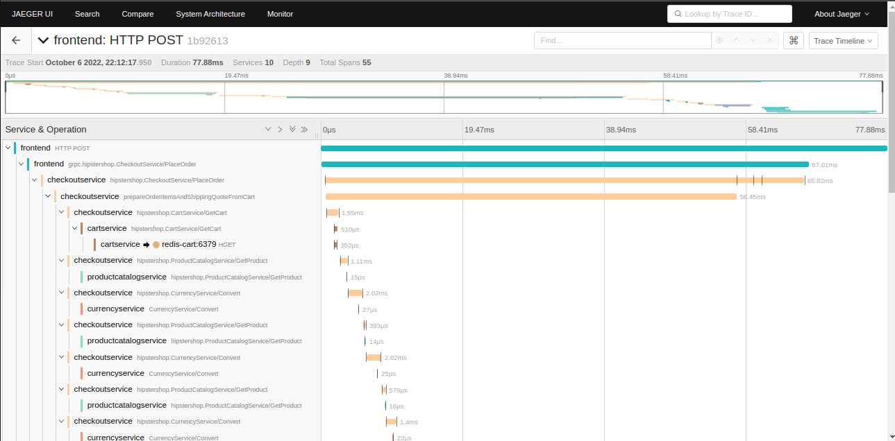
Our checkout request doesn't do its work alone. It arrives at a gateway (the front door that receives requests and passes them on), which calls the checkout service, which calls an inventory service, and any of them may be where the time went. A metric can tell us the checkout endpoint's p99 went from 200 ms to 4 seconds. A log line from checkout only knows checkout's total. We need a record that follows one request through every service it touches, and shows how long each step took. A trace of one slow checkout can show, for instance, that 3.7 of those seconds were a single call to the inventory service, waiting on a lock.
7.1Spans and trace context
A span is one timed operation: a request handled, a query run, a call made. It has a start, a duration, a parent, and attributes, key-value details such as the route or the customer ID. The spans of one request form a tree, because the gateway's span has the checkout call as a child, which has the inventory call as a child. That tree is a trace, and all of its spans share one trace ID.
For that to work across services, each call has to carry the trace ID and the caller's span ID to the next service, so the next service can attach its span in the right place. The standard way is the W3C Trace Context traceparent header, an extra line in the HTTP request:
traceparent: 00-4bf92f3577b34da6a3ce929d0e0e4736-00f067aa0ba902b7-01
             │  │                                │                └ flags: 01 = sampled
             │  │                                └ parent span ID (8 bytes)
             │  └ trace ID (16 bytes)
             └ version
The flags field says whether this request is being recorded in full, called being sampled, and 7.2 explains who decides that and why. Here is our checkout request going through three services:
traceparent on the incoming request, so the gateway starts a new trace: it generates a 16-byte trace ID and makes the sampling decision.Look at the last two messages. Each service reports only its own spans, to a collector, a separate program that receives spans and passes them on. The whole trace exists only after the collector or a backend behind it joins the spans by trace ID, so whatever does the joining needs all the spans of a trace. That comes back in 7.3.
?Why does one uninstrumented service break the whole trace?
Because propagation is hop by hop. A service is instrumented when it has tracing code that reads the incoming traceparent and writes it on outgoing calls. If a service in the middle isn't instrumented, the services after it start new traces. You get two half-traces with no link between them. Proxies, queues and thread pools are the usual culprits: the context has to be carried across every asynchronous hand-off, too.
7.2Too many traces: head sampling
Recording a span for every operation in every service, and exporting all of them, is expensive, in the same way that logging every request was in section 2. Most systems record only a share of requests, and choosing the share is called sampling. The simplest way is head sampling: the decision is made at the very start of the request, at the root span, and passed down in the traceparent flags so that every service agrees. It's cheap, because an unsampled request records nothing anywhere.
Dapper, Google's tracing system, started this way. Its 2010 paper describes a first production version averaging one sampled trace for every 1,024 candidates.
The weakness is that the decision is made before anything interesting has happened. At 1 in 1,024, a failure that affects one request in 10,000 is captured about once every ten million requests. Our customer's four-second request had a 1-in-1,024 chance of being kept, and the sampler didn't know it was slow when it decided. We'd like to decide after the request has finished.
7.3Deciding afterwards: tail sampling
Tail sampling decides after the trace is complete: keep every trace with an error, every trace slower than a threshold, and a small share of the rest. The most common tracing toolkit is OpenTelemetry, an open standard with libraries for every major language plus a collector program of its own. The OpenTelemetry Collector has a tail sampling processor that does this, with policies such as status_code, latency, probabilistic and rate_limiting. Here is what it does with three checkout requests, one of them ours:
4bf9…, which took 3.7 s.The two sampling methods trade against each other:
| Head sampling | Tail sampling | |
|---|---|---|
| Decides | At the root span, before the work | After the trace completes |
| Cost when dropped | Nearly zero in every service | Every span is created, exported and buffered |
| Keeps errors and slow traces | Only by chance | By policy |
| Infrastructure | Nothing extra | Collectors that see whole traces, with memory to buffer them |
?Why does tail sampling need two layers of collectors?
Because a decision about a trace needs every span of it, and spans arrive from many services at different collectors. The processor's README says all spans of a trace "MUST be received by the same collector instance". The standard deployment is a first layer running the load-balancing exporter, which routes by trace ID, in front of a second layer running tail sampling. The second layer buffers every trace for decision_wait (30 s by default) and holds up to num_traces (50,000 by default) in memory.
7.4Inside the OpenTelemetry SDK
Sampling decisions and exporting happen inside each service, in a library. OpenTelemetry splits that library into an API (what other libraries call to create spans, and a no-op if nothing's installed) and an SDK (what the application installs to sample, batch and export them). A span's path out of the process:
tracer.Start(ctx, "POST /api/v1/orders"). The API asks the SDK for a span, passing the parent context from ctx.The design decision that matters most is what happens when that queue is full. In opentelemetry-go, by default, the span is dropped and counted:
func (bsp *batchSpanProcessor) enqueueDrop(ctx context.Context, sd ReadOnlySpan) bool {
	if !sd.SpanContext().IsSampled() {
		return false
	}

	select {
	case bsp.queue <- sd:
		return true
	default:
		atomic.AddUint32(&bsp.dropped, 1)
		/* ... self-observability counter, error type queueFull ... */
	}
	return false
}
The select tries to put the span on the queue. If the queue has room it succeeds, and if not, the default branch runs: it adds one to a dropped-spans counter and gives up without waiting.
?Why drop spans instead of waiting?
Because telemetry must never take the service down with it. If the exporter is slow or the collector is unreachable, blocking would make every request wait on the tracing pipeline. The SDK spec defines the defaults (queue 2,048, batch 512, delay 5,000 ms, timeout 30,000 ms) and says plainly that once the queue is full, "spans are dropped." There's a WithBlocking() option for the rare case where losing spans is worse than latency.
We now have three signals that each hold part of the story about one request. The last question is how to get from one to the next.
08Using the signals together
8.1From a spike to the customer's request
Each jump needs something the two signals share. The link from metrics to traces is an exemplar: a trace ID attached to one observation in a histogram bucket.
http_request_duration_seconds_bucket{le="0.5"} 1204 # {trace_id="4bf92f3577b34da6a3ce929d0e0e4736"} 0.43The part after the # is an extension of the scrape format called OpenMetrics: one example observation of 0.43 seconds, and the trace it came from. A dashboard can show it as a dot on the latency graph that links straight to that request's trace. In Prometheus 3.9.1, storing exemplars still needs --enable-feature=exemplar-storage. The link from traces to logs is the trace_id field on every log line, and the link from logs back to metrics is using the same names for the same things: route, status, service.
Now go back to our customer and see what each signal did:
| Step | You look at | You learn |
|---|---|---|
| 1 | The latency histogram on the dashboard | The p99 for checkout jumped from 200 ms to 4 s (section 6). The average hid it. |
| 2 | The exemplar dot on the spike | A trace ID of a slow request, such as 4bf9… |
| 3 | That trace | 3.7 s of it was one call to the inventory service, waiting on a lock (section 7) |
| 4 | The logs, searched for that trace_id | The full line: status 201, duration_ms 3712, customer_id c_81723 (section 2) |
Notice that we never scanned 22.6 GB of logs. The counts were cheap enough to keep for every request, so they showed the spike. The exemplar turned the spike into one trace ID, tail sampling had kept that trace because it was slow, and the final log search was a lookup by one ID.
8.2What to measure first
You can't instrument everything at once, so two checklists cover most services. RED, for anything that serves requests: Rate, Errors, Duration. USE, from Brendan Gregg, for anything that is a resource: Utilisation, Saturation, Errors.
| Thing | Method | The three metrics |
|---|---|---|
| HTTP or RPC service | RED | Requests/s by route; error ratio; latency histogram |
| Queue consumer | RED | Messages/s; failures; processing time, plus queue age |
| Connection pool | USE | In use / size; waiters and wait time; timeouts |
| Disk, CPU, NIC | USE | Busy %; queue depth or run queue; device errors |
Alert on the RED metrics users feel, through SLO burn rates (chapter 40 explains these), and use the USE metrics to explain the alert once you're looking.
09Running it in production
9.1Commands for the questions this chapter raised
Each question has a query or a tool that answers it on a running system.
# Is every target being scraped? (section 3.2)
up == 0

# How many series are there, and is the count growing? (section 5)
prometheus_tsdb_head_series
rate(prometheus_tsdb_head_series_created_total[5m])

# Which metric names have the most series? Which label has the most values? (section 5.3)
topk(10, count by (__name__) ({__name__=~".+"}))
count(count by (customer_id) (http_requests_total))

# What is the p99 across all replicas? (section 6.1)
histogram_quantile(0.99, sum by (le) (rate(http_request_duration_seconds_bucket[5m])))# Which labels have the most values and the highest churn in stored data? (section 5.3)
promtool tsdb analyze <data-dir>
# Are exemplars being stored for the dashboard dots? (section 8.1)
prometheus --enable-feature=exemplar-storage ...9.2Rules that hold up
- Alert and graph on metrics; use logs and traces for detail. The same service differs by about 4,000 times in volume between logs and metrics.
- Bound every label. A label's values should be something you could list: routes, status classes, tiers. Never a raw path or an ID.
- Use histograms, not summaries, and put a bucket boundary at your SLO threshold.
- Use at least four scrape intervals as the
rate()range, and never userate()on a gauge. - Put
trace_idon every log line, and use a ParentBased sampler in every service so a trace is kept whole or dropped whole. - Let telemetry drop under load; don't block on it. Count what's dropped and watch the counter.
9.3What you trade for what
| You get | You pay | When the bill arrives |
|---|---|---|
| Counters whose cost doesn't depend on traffic | No per-request detail, and every label must be bounded | When you need to know which customer was affected |
Pull-based scraping, so a dead service shows as up 0 | Short-lived jobs and targets Prometheus can't reach need a Pushgateway or remote_write | As batch jobs whose metrics never arrive |
| About 2 bytes per sample from Gorilla | The timing has to stay regular | As storage that nearly doubles when scrape timing jitters |
| Histograms that add across replicas | Percentiles are interpolated estimates | As a p99 that's 22–52% off with wide buckets |
| Full detail in every log line | Storage and ingest for every event | As 22.6 GB a day at 1,000 requests a second |
| Cheap head sampling | Rare failures are mostly missed | A failure that hits 1 request in 10,000 captured about once per ten million |
| Tail sampling that keeps errors and slow traces | Collectors with memory for whole traces, plus a routing layer | As memory for up to 50,000 buffered traces per collector |
9.4Symptom, cause, fix
| Symptom | Likely cause | Fix |
|---|---|---|
| Prometheus OOM-killed, or memory climbing | Series count grew: a new high-cardinality label, or pod churn | topk by __name__, promtool tsdb analyze; drop or relabel |
| Slow dashboards, query timeouts | Regex matchers on high-cardinality labels; long ranges over raw series | Recording rules; equality matchers; fewer series |
Gaps in rate() graphs | Range shorter than about 4 scrape intervals | Use at least [1m] at a 15 s interval |
| p99 on the dashboard doesn't match user reports | Wide histogram buckets; or averaged summaries | Bucket at the SLO threshold; native histograms; never average quantiles |
| Traces broken into pieces | A hop not propagating traceparent (proxy, queue, thread pool) | Instrument the hop; carry context across async hand-offs |
| Spans missing under load | Batch processor queue full; spans dropped | Raise queue size, export faster, check the dropped-span count |
| Tail sampling keeps partial traces | Spans of one trace reaching different collectors | Load-balancing exporter by trace ID in front |
| Logging bill doubling | Debug level left on, or logs in a hot loop | Runtime-switchable levels; sample successes by trace ID |
10Summary
- An average can be accurate and still hide the slow requests. With 1% of requests slow, the mean was double the median and matched no request.
- Logging every request answers "what happened to this one", at a price. At 1,000 requests a second that's about 22.6 GB a day, and a question about the whole needs a scan of millions of lines.
- A Prometheus series is a name plus a label set. Every new combination of label values is a new series with its own storage, and a counter costs the same at any traffic.
- Pull makes absence visible. A failed scrape sets
upto 0; a dead pusher just goes quiet. - A sample goes head, then WAL, then chunk, then block. The head is in memory, and the log on disk lets a crash be replayed.
- Gorilla encoding makes regular data cheap. A perfectly regular timestamp costs one bit; counters cost 1.87 bytes a sample, jittered ones 3.71, random floats 7.98. Together with counting instead of recording, that makes a service's metrics about 4,000 times smaller than its logs.
- Postings lists make label queries fast. Selectors intersect sorted lists of series IDs; regexes over huge label sets don't.
- Cardinality is the bill. Each active series costs about 2.9 KB of RAM, and one unbounded label can multiply a metric 10,000×.
- Histogram percentiles are interpolations. With default buckets the p99 was off by 22–52%; put a boundary at your SLO threshold.
- A trace follows one request across services. The
traceparentheader carries the trace ID hop by hop, and one hop that drops it splits the trace. - Head sampling is cheap, tail sampling is smart. Tail sampling needs every span of a trace at one collector, so it needs a routing layer, and an exemplar and the trace ID in the log join the three signals back together.
11Build this
A cardinality lab.
- Run Prometheus locally with a static
/metricsfile you generate, as in section 5.2. Measure RSS at 10k, 100k and 500k series and fit a per-series cost for your version. - Add a label with high churn (a new value every scrape) and watch
prometheus_tsdb_head_seriesand memory until the next head compaction. - Write a histogram with default buckets and one with a boundary at your SLO, feed both the same latencies, and compare
histogram_quantile(0.99, …)and the fraction under the threshold against the truth. - Instrument two small services with OpenTelemetry, break propagation in one hop, and find the split trace in the backend.
12Interview questions
beginnerWhat's the difference between a counter and a gauge, and why does it matter for rate()?›
A counter only increases, except for resets to zero on restart. A gauge goes up and down. rate() treats any decrease as a counter reset, adding the new value to the increase, so on a gauge every drop is misread as a restart. Use rate() and increase() on counters, and deriv() or delta() on gauges.
beginnerWhy shouldn't you put a user ID in a Prometheus label?›
Every unique combination of label values is a separate series, stored and indexed separately in memory. A user ID multiplies the series count by the number of users. In Prometheus 3.9.1 each active series costs about 2.9 KB of RAM, so ten million series is roughly 29 GB. Put per-user detail on logs and traces instead, where a new value adds a line or a span and not a whole series.
intermediateWhy can you aggregate histograms across instances but not summaries?›
A histogram exports counts per bucket, and counts add: sum the buckets across instances and compute the quantile from the total. A summary exports quantiles already computed per instance, and quantiles don't combine; the average of ten p99s isn't the p99 of anything.
intermediateHow does Prometheus compress samples?›
With Gorilla's scheme. Timestamps are stored as delta-of-delta, so a perfectly regular scrape costs one bit per sample, with larger bit buckets for jitter (14, 17, 20 or 64 bits plus a prefix, since Prometheus uses milliseconds). Values are XORed with the previous value and only the meaningful bits are stored. Chunks hold about 120 samples. Real counters come out near 2 bytes per sample, and random floats take about 8.
intermediateHow does a trace ID get from one service to the next?›
In the W3C traceparent header: version, 16-byte trace ID, 8-byte parent span ID and flags, where the low bit means sampled. Each service reads it from the incoming request, creates its own span as a child, and writes a new traceparent with the same trace ID and its own span ID on outgoing calls. Each service exports its own spans; the backend joins them by trace ID.
deepWhat's the trade-off between head and tail sampling?›
Head sampling decides at the root and propagates the decision, so dropped traces cost almost nothing, but it can't know which requests will fail or be slow. Tail sampling decides after the trace is complete, so it can keep every error and slow trace, but every span must be created and exported, and all spans of a trace must reach the same collector, which needs a load-balancing layer routing by trace ID and memory to buffer traces for the decision wait.
deepA dashboard p99 says 190 ms, but users report 130 ms. What's going on?›
Probably histogram interpolation. histogram_quantile() assumes observations are spread evenly inside the bucket that holds the target rank, so if p99 falls in a wide bucket such as 100–250 ms the estimate can land far from the truth. With default buckets and a log-normal distribution the true p99 was 123 ms and the estimate 187 ms. Add bucket boundaries near the values you care about, especially the SLO threshold, or use native histograms.
deepWhy does the OpenTelemetry batch span processor drop spans instead of blocking?›
So that the tracing pipeline can't add latency to or take down the service. If the exporter is slow or the collector unreachable, blocking on a full queue would make request threads wait on telemetry. The spec's defaults (queue 2,048, batch 512, 5 s delay) bound memory, and overflow is counted as dropped. Blocking is available as an opt-in for the rare cases where completeness matters more.
13Go deeper
Your metric has labels with 4, 20 and 300 values. What's the most series it can have?›
24,000: 4 × 20 × 300. Labels multiply.
Scrapes run every 15 s but arrive with ±50 ms jitter. What happens to storage?›
The delta-of-delta is almost never zero, so each timestamp costs 16 bits instead of 1. For a counter that takes it from 1.87 to 3.71 bytes a sample.
Where does histogram_quantile() put p99 if it lands in the +Inf bucket?›
At the highest finite bucket bound. It can never report a value above your largest bucket.
Why use a ParentBased sampler in every service?›
So a child follows its parent's decision. Otherwise services sampling independently keep different subsets of the same traces, and most kept traces are incomplete.
Delta-of-delta timestamps and XOR values, with the distribution data that justifies each. PDF
The design note behind Prometheus 2's storage: blocks, the head, the WAL and postings. archived copy
The paper most tracing systems descend from, including the case for sampling. PDF
The chunk encoding, head block and quantile code quoted here. v3.9.1
When to use which, and a worked example of interpolation error. prometheus.io
Samplers, span processors and their defaults. opentelemetry.io
The traceparent and tracestate headers, byte by byte.
w3.org
14Related chapters
What to do with these signals: SLIs, error budgets and burn-rate alerts. Chapter 40.
Why percentiles don't average, and how load generators hide the tail. Chapter 16.
Telemetry without changing the application: kernel tracing, off-CPU profiling and packet drops. Chapter 48.
Where observability goes in a design, and the numbers to size it with. Chapter 38.