It's ten past nine on a Friday in Lisbon. Ana's children are finally asleep, and she sits down in front of the living-room TV and opens Netflix. She picks her own profile, not the kids' one, and the home page fills the screen. The first row is Continue Watching, with the crime series she started on Wednesday. Below it are rows called Top Picks for Ana, Because You Watched, Scandinavian Thrillers, Trending Now, and a few dozen more she'll never scroll down to. Each title has a picture on it, and for one of the films the picture is a close-up of an actor she has watched in three other films. She scrolls a little, reads one synopsis, and presses Play.
That page took about a second to appear, and it looks like a list of shows. But every part of it is a decision. Which forty or so rows, out of tens of thousands Netflix could make for her? In what order? Which titles go in each row, and which go first? Which of a few dozen pictures should stand for each title? And all of this has to be decided for a household account, where the person holding the remote tonight may not be the person who watched the cartoons yesterday. Netflix's own research says a typical member gives up after perhaps 60 to 90 seconds of looking, having considered 10 to 20 titles. If none of those catch her, she may switch off.
In this case study we'll design the system that builds Ana's page the way an engineer would: start with the simplest design, find exactly where it breaks, and fix it, one step at a time. The question we'll keep coming back to is this: when Ana turns on Netflix, how does it choose, in about a second, which rows, which titles and which pictures to show her, out of everything it could show? Along the way we'll go from predicted star ratings down to vectors, nearest-neighbour indexes, the exploration of slot-machine problems and the experiments that tell Netflix whether any of it works.
01What we're building, and how big
1.1What it has to do
The part of Netflix this chapter covers is the home page and the machinery behind it. Netflix itself calls almost everything on that page a recommendation, and the list of jobs is longer than you might expect:
- Rank titles for each member: for Ana, an ordering of the catalogue from most to least likely to be enjoyed.
- Fill rows: thematic groups like Scandinavian Thrillers or Because You Watched, each with its titles in a personal order.
- Choose and order the rows on the page, for her device.
- Pick the evidence for each title: which picture, which synopsis, whether to mention an award.
- Learn from what she does: plays, skips, abandonments, thumbs up and down, and feed it back.
- Measure whether a change made the service better, before it reaches everyone. The usual tool is an A/B test: give the change to a random group of members and compare them with a group that didn't get it (section 12).
And the qualities it needs:
- Relevant and diverse: rows that match Ana's tastes, but not forty variations of the same one, since tonight she might be in a different mood, or someone else in the house might be holding the remote.
- Fresh but stable: the page should react to the episode she finished last night, but she should still be able to find the film she noticed yesterday.
- Fast: the page is assembled while she waits, so there's a budget of a fraction of a second for the work done at request time.
- Available: if the clever parts fail, she still gets a reasonable page.
Notice the difference from the Uber case study. There, the hard question was physical: which of the moving cars is close to this point. Here the question is about taste, which nobody can observe directly, so the system has to infer it from behaviour and then check its guesses with experiments. Most of this case study is about doing that inference cheaply enough for every member, every evening.
1.2How big is it?
Netflix reported over 300 million members at the end of 2024, and its engineers describe "hundreds of billions" of recorded interactions from them. In 2015, two of Netflix's product leaders, Carlos Gomez-Uribe and Neil Hunt, described the home page as typically about 40 rows, with up to 75 titles in each, the numbers varying by device. They also wrote that a typical member has "tens of thousands of rows" that could go on their home page. The catalogue itself is "thousands of titles", as a 2017 Netflix post put it; Netflix doesn't publish an exact count per country.
Two more figures from that 2015 paper explain why Netflix invests so much here. Recommendations influence the choice behind about 80% of the hours streamed; the other 20% comes from search. And the authors estimated that personalisation and recommendations together save Netflix more than a billion dollars a year, mostly by keeping members who would otherwise cancel.
Ana's page has about 40 rows, chosen and ordered from, say, 10,000 candidate rows. Roughly how many different pages could the system build for her? Could it score each one and pick the best?
02Version 1: predict a star rating
2.1The obvious design
Go back to the mid-2000s, when Netflix mostly rented DVDs by post. Members rated films from one to five stars, and the natural design was: predict how many stars Ana would give each film she hasn't rated, and show her the films with the highest predictions. Netflix's system for this was called Cinematch.
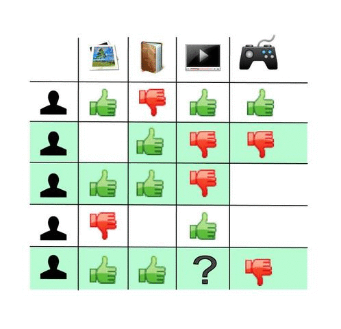
How do you predict a rating Ana hasn't given? Classically, you use other people. Find members whose past ratings agree with Ana's, and look at what they thought of the film in question. This idea is called collaborative filtering: the members, collectively, filter the catalogue for each other.
2.2The Netflix Prize
In 2006 Netflix turned this exact problem into a public competition. It released about 100 million anonymised ratings and offered a million dollars to the first team that could predict held-out ratings 10% more accurately than Cinematch. Accuracy was measured as root mean squared error (RMSE): take each prediction's error in stars, square it, average the squares, and take the square root. Cinematch scored 0.9525, so the target was 0.8572 or lower.
A year in, a team called Korbell won the first progress prize with an 8.43% improvement. They reported more than 2,000 hours of work and a final blend of 107 different algorithms. Netflix looked inside the blend and found two algorithms doing most of the work: one the community called SVD, a form of matrix factorisation (next subsection), with an RMSE of 0.8914 on its own, and one called a restricted Boltzmann machine, at 0.8990. A simple blend of the two reached 0.88. Netflix rebuilt both to handle its 5 billion ratings instead of the competition's 100 million, and put them into production.
In September 2009 a merged team, BellKor's Pragmatic Chaos, won the grand prize with a 10.06% improvement, a blend of hundreds of models. Netflix never shipped it. Its engineers wrote in 2012 that the extra accuracy they measured "did not seem to justify the engineering effort needed to bring them into a production environment". A planned second competition was cancelled in 2010 after a privacy lawsuit and concerns from the US Federal Trade Commission. Researchers had already shown that some members in the "anonymous" data could be identified by matching their ratings with public reviews on other sites.
2.3Matrix factorisation: a vector for every member and title
The algorithm that survived matters here, because the rest of the chapter grows out of it. Picture all the ratings as a huge table, members down the side and titles across the top, mostly empty because each member has rated a tiny fraction of the catalogue. Matrix factorisation assumes this table can be approximated by multiplying two thin tables: one with a short list of numbers for each member, and one with a short list of numbers for each title. Ana's predicted rating for a film is then the dot product of her list and the film's list: multiply them number by number and add up.
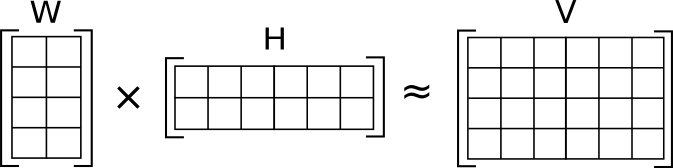
Nobody tells the algorithm what the numbers mean. It starts them at random and repeatedly nudges them so that the dot products match the ratings that do exist. This program does that for five people and six titles, with two numbers each. Ana hasn't rated the romantic comedy, and the program predicts what she'd give it:
import random
random.seed(7)

# Ratings 1-5 from five viewers for six titles; 0 means "hasn't rated it"
titles = ["Space Docs", "Heist", "Rom-com", "Baking", "Thriller", "Cartoon"]
R = {
    "Ana":   [5, 4, 0, 1, 5, 1],
    "Ben":   [4, 5, 1, 1, 4, 0],
    "Chloe": [1, 1, 5, 5, 0, 4],
    "Dev":   [0, 1, 4, 5, 1, 5],
    "Eve":   [5, 0, 1, 2, 5, 1],
}

K = 2                      # each viewer and title becomes a vector of 2 numbers
P = {u: [random.uniform(0, 1) for _ in range(K)] for u in R}
Q = [[random.uniform(0, 1) for _ in range(K)] for _ in titles]
dot = lambda a, b: sum(x * y for x, y in zip(a, b))

for epoch in range(3000):  # nudge the vectors to fit the known ratings
    for u, row in R.items():
        for i, r in enumerate(row):
            if r == 0:
                continue
            err = r - dot(P[u], Q[i])
            for k in range(K):
                pu, qi = P[u][k], Q[i][k]
                P[u][k] += 0.01 * (err * qi - 0.02 * pu)
                Q[i][k] += 0.01 * (err * pu - 0.02 * qi)

print("Ana's vector:", [round(x, 2) for x in P["Ana"]])
for i, t in enumerate(titles):
    known = R["Ana"][i]
    vec = [round(x, 2) for x in Q[i]]
print(f"{t:10} vector {vec} predicted {dot(P['Ana'], Q[i]):3.1f} actual {known or '?'}")Ana's vector: [2.02, 0.29]
Space Docs vector [2.25, 0.32] predicted 4.7 actual 5
Heist vector [2.23, 0.33] predicted 4.6 actual 4
Rom-com vector [0.11, 1.93] predicted 0.8 actual ?
Baking vector [0.29, 2.15] predicted 1.2 actual 1
Thriller vector [2.25, 0.32] predicted 4.6 actual 5
Cartoon vector [0.11, 1.94] predicted 0.8 actual 1Look at the title vectors. Without being told anything about genre, the program has put the documentary, the heist film and the thriller at roughly (2.2, 0.3), and the romantic comedy, the baking show and the cartoon at roughly (0.2, 2.0). Its first number has come to mean something like "tense, grown-up viewing" and the second "gentle, light viewing". Ana's vector is (2.02, 0.29), so she sits with the first group, and her predicted rating for the romantic comedy is 0.8, below the bottom of the scale (nothing in the arithmetic keeps predictions between 1 and 5). Real systems use tens or hundreds of numbers per vector, and the meanings are probably never this tidy, but the mechanism is the same.
2.4Where version 1 breaks
Version 1 has three problems, and each one drives a later section.
The first is that stars were the wrong target. Netflix launched streaming in 2007, a year into the prize. With DVDs, people chose carefully because a swap took days, and Netflix learned nothing about the viewing itself. With streaming, members sample a few titles, abandon some after ten minutes, binge others, and every one of those actions is recorded. Netflix's 2012 post says the focus moved from predicting ratings to everything else on the page, and by then 75% of what people watched came from some kind of recommendation. Stars became one weak signal among many. What to predict instead is section 6.
The second is that one ranked list isn't a page. Ana's household shares the account, her mood changes from evening to evening, and a single list with her top 40 predictions would probably be 40 tense thrillers. Building a page of rows is section 9, and choosing a picture for each title is section 10.
And third, there's cost. Predicting with two numbers per title is trivially cheap, but the models that replaced it are far richer, and running a rich model on every title for every member, every time someone opens the app, doesn't fit in the time budget. Before we can see why, we need a closer look at those vectors, because they turn out to be the tool that makes the whole system affordable.
03Members and titles as vectors
3.1Embeddings
The lists of numbers that matrix factorisation learned have a general name. An embedding is a vector of numbers learned for each thing in a large set, members, titles, genres, search words, so that things that behave alike end up with similar vectors. "Similar" is measured geometrically: either the dot product, or the cosine similarity, which is the cosine of the angle between two vectors and ignores their lengths. Two vectors pointing the same way have a cosine of 1; at right angles, 0.
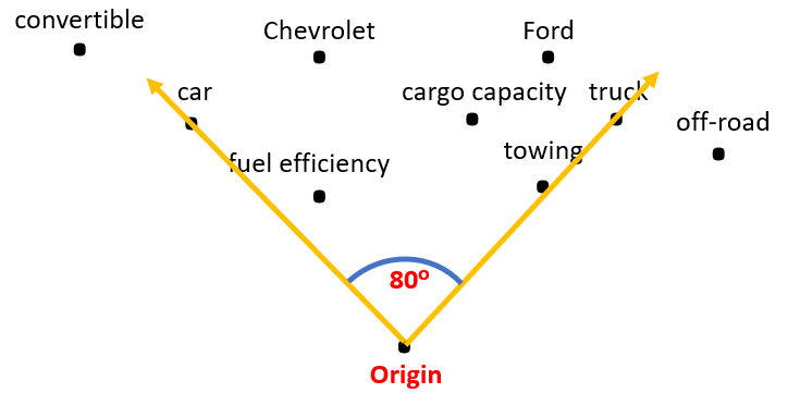
Embeddings turn questions about taste into geometry. "Which titles would Ana like?" becomes "which title vectors point the same way as Ana's?" "Which titles are like the crime series she's watching?" becomes "which title vectors are near that one?" That second question is what powers a Because You Watched row. Netflix's 2015 paper calls the algorithm behind those rows "sims": an unpersonalised list of similar titles for every title, with the choice of which Because You Watched rows reach Ana's page, and which of the similar titles appear in them, personalised.
3.2From matrix factorisation to two towers
Matrix factorisation gives each member one fixed vector, learned from their ratings. Two things are wrong with that for Ana. Her vector should depend on more than ratings: what she watched in the last hour, the device, the time of day. And a brand-new member, or a title released this morning, has no history at all, so it has no vector. This is the cold-start problem.
Instead, compute each vector from features, facts about the member or title such as recent viewing or genre, using a neural network: a function with millions of adjustable numbers, tuned from examples the same way the TryIt tuned its vectors. One network, the member side, takes everything known about Ana and her context and outputs her vector. A second network, the title side, takes a title's ID and its metadata (genres, cast, language, tone) and outputs its vector. Ana's score for a title is still the dot product of the two. This shape is called a two-tower model, after the two networks side by side. Its useful property is that the title tower doesn't depend on Ana, so every title's vector can be computed ahead of time, in a batch job, and only her side needs computing when she opens the app.
Netflix described exactly this kind of cold-start handling in its 2025 post on a foundation model for recommendations (section 13 returns to it). Each title's final embedding mixes a learned ID embedding with an embedding built from metadata, and the mix depends on the title's age: a title launched today leans on its metadata, an established one on what members did with it. Those title and member embeddings are computed in batch jobs and stored, and the post says they're used for candidate generation, retrieving appealing titles for a member, and for title-to-title recommendations.
04Why the system is a funnel
4.1The cost of scoring everything well
A dot product between two vectors of 64 numbers costs 64 multiplications and additions, a few dozen nanoseconds. Doing that for every title in a catalogue of thousands takes microseconds. So the cheap score is cheap. Trouble is, the cheap score isn't good enough to put titles in their final order.
The best predictions come from models that look at hundreds of features of the pair, Ana and this particular title: how many episodes of this show she's watched, how long since she last watched anything from this genre, how often the title has been shown to her without a play, how popular it is this week in Portugal. Those features exist only for the pair, so they can't be precomputed per title, and the model that combines them is far bigger than a dot product.
YouTube's 2016 ranking network had hidden layers of 1,024, 512 and 256 units. Suppose its input is about 1,000 numbers. Roughly how much arithmetic is one prediction, and what would it cost to run it on 5,000 titles for one page? What about YouTube's millions of videos?
4.2Candidate generation, ranking, and the page
The standard answer is a funnel: a sequence of stages, each one cheaper per item than the next, each one passing on fewer items. YouTube's 2016 paper drew it as millions of videos narrowed by candidate generation to hundreds, then ranked by a heavier model to the dozens that appear. A third stage, often called re-ranking, then applies rules and page-level concerns: no two titles too alike next to each other, nothing already watched, a mix of familiar and new.
Netflix's shape differs from YouTube's in an instructive way. Its catalogue is small enough that, according to the 2015 paper, the personalised video ranker behind genre rows "orders the entire catalog of videos ... for each member profile". With thousands of titles, a full ordering per profile can be computed ahead of time, in batch. The funnel still exists, but its wide end is somewhere else: the tens of thousands of candidate rows, and the combinations of rows, titles and pictures on a page. YouTube's is wide at the item level because it has millions of videos.
Where should the expensive scoring happen?
- No model latency at request time
- Can afford heavy models
- Stale until the next run
- Can't use tonight's context: device, time, last hour
- Fully fresh and contextual
- Seconds of CPU per page
- Impossible for large catalogues
- Fresh where it matters
- Fits a request budget
- Several systems to keep consistent
- A title missed by candidate generation can never be ranked
Every large recommender ends up mixing these, and Netflix's 2013 architecture post (section 7) says so directly: the bulk of recommendations can be computed offline, with freshness added by post-processing the lists online using real-time signals. Netflix hasn't published the exact split for each row type on today's page.
05Finding the nearest vectors quickly
5.1When a scan stops being enough
Candidate generation's main tool is "find the title vectors nearest to this vector". For Netflix's catalogue alone, checking every title is fine: a few thousand dot products. But the same question shows up at much larger sizes. YouTube's 2016 paper describes scoring "millions of items under a strict serving latency of tens of milliseconds"; Pinterest's graph has billions of pins; and within Netflix, the 2025 foundation-model post says its embeddings serve both candidate retrieval and title-to-title similarity across the whole catalogue. Netflix hasn't published which nearest-neighbour index it uses, if any, so this section covers the techniques any design at this scale would reach for.
Finding the exact nearest vectors in many dimensions turns out to have no shortcut that beats scanning by much. Tree structures that work well for two-dimensional maps, like the quadtrees in the Uber case study, stop helping once there are more than about ten dimensions. So large systems settle for approximate nearest-neighbour (ANN) search: return most of the true nearest neighbours, quickly, and accept missing a few. Quality is measured as recall: of the true 10 nearest, how many did the search return? YouTube's paper adds a reassuring detail: its A/B results "were not particularly sensitive to the choice of nearest neighbor search algorithm".
There are two families of ANN index in wide use, both implemented in Faiss, the open-source library Facebook (now Meta) released in 2017: inverted files and graphs.
5.2Inverted files: search only the nearby clusters
The first idea is the same as the Uber chapter's grid, adapted to many dimensions. Before any search, group the title vectors into clusters with k-means: pick a few hundred centre points, assign each vector to its nearest centre, move each centre to the average of its vectors, and repeat. Each cluster's vectors are stored together in a list. At search time, compare the query with the centres first, then scan only the lists of the few nearest clusters. Faiss calls this an inverted file (IVF); the number of clusters is nlist and the number searched is nprobe.
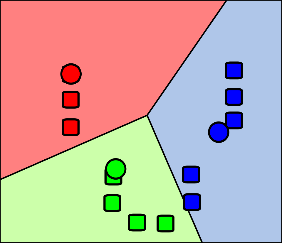
The catch is the edges. A query near the border of its cluster may have true neighbours sitting in the cluster next door, which is why nprobe is more than 1. This program builds an inverted file over 20,000 vectors in 16 dimensions, bunched around 40 "tastes", and measures how many true nearest neighbours it finds as it searches more lists:
import random
random.seed(3)
D, N, LISTS = 16, 20_000, 100

# 20,000 title vectors in 16 dimensions, bunched around 40 "tastes"
tastes = [[random.gauss(0, 1) for _ in range(D)] for _ in range(40)]
def near(c): return [x + random.gauss(0, 0.9) for x in c]
titles = [near(random.choice(tastes)) for _ in range(N)]
queries = [near(random.choice(tastes)) for _ in range(50)]

def d2(a, b): return sum((x - y) ** 2 for x, y in zip(a, b))

# Build the inverted file: 100 centroids (two rounds of k-means),
# then each vector goes in the list of its nearest centroid
cents = random.sample(titles, LISTS)
for _ in range(2):
    groups = [[] for _ in range(LISTS)]
    for v in titles:
        groups[min(range(LISTS), key=lambda c: d2(v, cents[c]))].append(v)
    cents = [[sum(col) / len(g) for col in zip(*g)] if g else cents[i]
             for i, g in enumerate(groups)]
lists = [[] for _ in range(LISTS)]
for idx, v in enumerate(titles):
    lists[min(range(LISTS), key=lambda c: d2(v, cents[c]))].append(idx)

def exact(q, k=10):
    return set(sorted(range(N), key=lambda i: d2(q, titles[i]))[:k])

def ivf(q, nprobe, k=10):
    probe = sorted(range(LISTS), key=lambda c: d2(q, cents[c]))[:nprobe]
    cand = [i for c in probe for i in lists[c]]
    return set(sorted(cand, key=lambda i: d2(q, titles[i]))[:k]), LISTS + len(cand)

truth = [exact(q) for q in queries]
print(f"exact scan: {N:,} distances per query, recall 100%")
for nprobe in (1, 4, 16):
    hits = work = 0
    for q, t in zip(queries, truth):
        found, cost = ivf(q, nprobe)
        hits += len(found & t); work += cost
    print(f"IVF nprobe={nprobe:2}: {work // len(queries):6,} distances per query, "
f"recall {hits / (10 * len(queries)):.0%}")exact scan: 20,000 distances per query, recall 100%
IVF nprobe= 1: 360 distances per query, recall 55%
IVF nprobe= 4: 925 distances per query, recall 86%
IVF nprobe=16: 3,217 distances per query, recall 99%Read the three IVF lines as a dial. Searching one list costs 360 distance computations, the 100 centres plus about 260 vectors, which is 55 times less work than the scan, but finds only 55% of the true neighbours. Searching 16 lists finds 99% of them for about a sixth of the scan's work. That trade between speed and recall is the main tuning decision in any ANN index. The Faiss paper gives the rule of thumb behind the list count: with nprobe fixed, the distance computations per query are about nlist + nprobe × N / nlist, which is smallest when nlist is around the square root of nprobe × N.
5.3Product quantisation: making vectors small
Speed isn't the only limit; memory is the other. A vector of 128 floating-point numbers takes 512 bytes, so a billion of them take half a terabyte. Product quantisation (PQ) compresses each vector. Cut it into, say, 16 pieces of 8 numbers. For each piece position, run k-means over all vectors' pieces to find 256 typical pieces, and store each vector as 16 one-byte numbers saying which typical piece is closest in each position. Each vector shrinks from 512 bytes to 16, 32 times smaller.
Distances get cheaper too. For a query, precompute a table of the distance from each of its 16 pieces to each of the 256 typical pieces. Approximate distance to any stored vector is then 16 table lookups and additions. Combining the two ideas, an inverted file whose lists hold PQ codes, is called IVF-PQ, and it's how Faiss handles collections far beyond memory. The Faiss paper (2024) describes an index of 1.5 trillion vectors, compressed to 54 bytes each and spread over many servers, answering a query in about a second.
5.4Graphs: HNSW
The other family doesn't cluster at all. It links each vector to a handful of its near neighbours, making a graph, and searches by walking: start somewhere, look at the current node's neighbours, move to whichever is closest to the query, and repeat until no neighbour is closer. On its own, that walk is slow on a big graph, because it takes many short steps to cross it.
Hierarchical Navigable Small World (HNSW) graphs, published by Yury Malkov and Dmitry Yashunin in 2016, fix that with an idea borrowed from a much older data structure, the skip list. A skip list is a sorted linked list with extra "express lanes": every element is in the bottom lane, and each element is also promoted to the lane above with some fixed probability, so higher lanes are sparser. A search runs along the top lane until it would overshoot, drops a lane, and repeats.
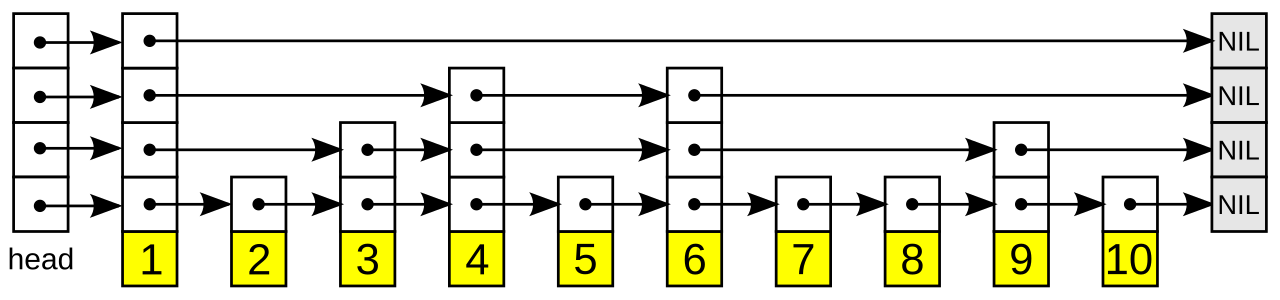
HNSW builds a stack of graphs the same way. Every vector is in layer 0. When a vector is inserted, it's given a top layer drawn at random, with each higher layer exponentially less likely: the paper picks the level as the floor of −ln(u) × mL, where u is a random number between 0 and 1 and mL = 1/ln(M). In each layer it's linked to up to M nearby vectors (2M in layer 0). The upper layers are sparse and their links are long; the bottom layer is dense and its links are short.
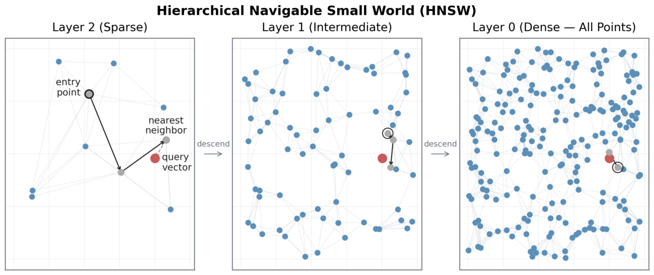
Two parameters set the trade. M, the number of links per node, sets memory and accuracy; the paper suggests values from about 5 to 48, which means roughly 60 to 450 bytes of links per vector on top of the vector itself. And ef, the size of the best-so-far list during search, is HNSW's equivalent of nprobe: raise it for higher recall, lower it for speed. It's the hierarchy that makes the number of steps grow roughly with the logarithm of the collection size, so a collection a thousand times larger needs only a few more hops.
Which index for candidate retrieval?
- Perfect recall
- Nothing to build or tune
- Fine for thousands of items
- Cost grows linearly with the collection
- Very compact: tens of bytes per vector
- Scales to billions and beyond
- Compression loses some accuracy
- Clusters need retraining as data drifts
- High recall at low latency
- Easy to add vectors one at a time
- Links cost memory per vector
- Deleting vectors is awkward
None is chosen here because the right one depends on size. For a catalogue the size of Netflix's, an exact scan is often the honest answer: it's exact, cheap and has nothing to go stale. HNSW is the common choice when a few million vectors fit in memory and latency matters; IVF-PQ when they don't fit. What Netflix runs in production is unpublished.
06What should the ranker predict?
6.1Plays, watch time, or something better
Candidate generation hands the ranker a few hundred titles for Ana. Now the ranker has to put them in order, which means it has to predict something, and section 2 showed that star ratings were the wrong something. An obvious replacement is the probability that she presses Play, which is called the take rate when measured: plays divided by impressions.
Optimise only for that, though, and the system learns to favour titles that are easy to start and disappointing to watch. YouTube's 2016 paper says it bluntly: ranking by click-through rate "often promotes deceptive videos that the user does not complete ('clickbait')". YouTube's answer was to predict expected watch time instead, using a neat trick. It trained an ordinary click predictor, but weighted each clicked example by how long the person watched; the odds the model learns then approximate expected watch time. Weighting every example equally made its watch-time loss 4.1% worse.
Netflix's 2024 post on long-term satisfaction goes a step further. Its aim is retention, members staying because they value Netflix enough to keep paying, but retention is useless as a direct training signal: it's noisy, it only moves for members close to cancelling, it's hard to attribute to any one recommendation, and it arrives once a month per account. So Netflix trains towards a proxy reward, a score computed from what a member did with a recommendation, engineered to line up with long-term satisfaction. The post's examples: finishing a season in a day is a strong positive; finishing a show over several weeks and then giving it a thumbs-down is a negative despite all the hours; ten minutes of a film is ambiguous; branching into a new genre after one show is especially valuable.
?What if the best evidence arrives weeks later?
Completion and thumbs often come days or weeks after the recommendation, and waiting that long to retrain leaves the model stale. Netflix's answer is a second model that predicts the delayed feedback from what has been observed so far, so training examples can be scored with "observed plus predicted" feedback shortly after the recommendation. That gives two kinds of model: delayed-feedback predictors used only offline, during training, and the recommendation policy that runs online.
What should the ranking model optimise?
- Clean, well-studied target
- Easy offline evaluation
- Few members rate
- Ratings don't predict what people actually watch
- Lots of data
- Directly about the page
- Rewards clickbait
- Ignores whether the viewing was any good
- Aligned with retention
- Sensitive to individual recommendations
- The reward itself must be designed and tested
- Better offline models can lose A/B tests if the reward is misaligned
Netflix moved along this list over a decade: stars until the prize, plays and engagement through the 2010s, and an explicit proxy-reward practice described in 2024. It calls the process reward engineering, by analogy with feature engineering: form a hypothesis, define a new proxy, train, and A/B test. The post also warns that improved models sometimes score better offline and flat or worse online, and treats that as a sign that the proxy needs fixing.
6.2Several objectives, one score
In practice a ranker predicts several things at once, the chance of a play, of finishing, of a thumbs-up, of abandoning, and the page needs one number per title to sort by. Simplest is a weighted sum, with weights set by hand and tuned with experiments. Netflix's weights are unpublished, but Twitter published its own in 2023, which makes a vivid example.
| Predicted engagement (Twitter/X, April 2023) | Weight |
|---|---|
| Likes the post | 0.5 |
| Reposts it | 1.0 |
| Replies | 13.5 |
| Replies, and the author engages with the reply | 75.0 |
| Opens the author's profile and likes or replies | 12.0 |
| Clicks into the conversation and stays 2 minutes | 10.0 |
| Says "show less", blocks or mutes | −74.0 |
| Reports the post | −369.0 |
The heavy ranker, a network of about 48 million parameters, outputs ten probabilities, and the score is the weighted sum. Twitter's notes say the weights were first set so that each term contributed about equally on average, then adjusted over time "to optimize for platform metrics". You can see how much product judgement lives in those numbers: a predicted report outweighs hundreds of predicted likes.
A ranker trained to maximise plays is replaced by one trained on a proxy reward that counts completions and thumbs-up. In an A/B test, what's most likely to happen first?
07Where the computation happens
7.1Offline, nearline and online
So far we've needed three kinds of work: training models on everyone's history, precomputing things like title embeddings and broad rankings, and the request-time work of retrieving and ranking for Ana right now. Netflix's 2013 post by Xavier Amatriain and Justin Basilico describes the architecture as three modes of computation, and the names have stuck.
Offline computation runs in batch over large data with relaxed deadlines: model training, and precomputing results to be served later. It can afford complex algorithms, but its results go stale between runs. Online computation runs while the member waits, so it can use the latest context, but it's bound by a response-time agreement and must have a fast fallback, such as a precomputed result. Nearline sits between: it runs online-style computations in response to events, but stores the results instead of serving them immediately. The post's example is the one Ana triggered last night: updating her recommendations to reflect that she started watching a series, right after she started.
In 2013 the event flow ran through an internal system called Manhattan, which the post compares to Twitter's Storm; logs went through Chukwa into Hadoop; results were published with an internal publish-subscribe tool called Hermes and stored in Cassandra, EVCache (Netflix's memcached-based cache) and MySQL. Those specific tools have probably all changed since, as tools do; the three-mode split is the durable part.
7.2Training every minute: ByteDance's Monolith
How fresh can the model itself be? Netflix's models are mostly trained offline, as the 2013 post says, with some online learning. ByteDance, which owns TikTok, published a design in 2022 that pushes freshness much further, for workloads like short-video ranking where interests shift within minutes. The paper describes the system's use in BytePlus Recommend, ByteDance's recommendation product for other businesses; whether TikTok's own feed runs on it isn't stated.
Monolith keeps training after deployment. User actions and features flow through Kafka, a Flink job joins each action to the features that were shown, and training workers consume those examples continuously. Every minute or so, the embeddings that changed since the last sync are copied from the training servers to the serving servers; the paper's example is 100,000 updated IDs with 1,024-number embeddings, about 400 MB a minute. Dense layers of the network change slowly, so they're synced once a day. On a public ads dataset, syncing every 30 minutes beat syncing every 5 hours, and both beat a model trained only in batch.
The other half of the paper is a data structure. Embedding tables for users and items are enormous, and the common shortcut is to hash IDs into a fixed-size table, accepting that some IDs share a vector. Monolith's authors measured the harm and instead built a collisionless table on cuckoo hashing: two tables, two hash functions, and every key lives in exactly one of its two possible slots. Inserting a key that finds its slot taken evicts the occupant to its other slot, which may evict another, until everything settles.
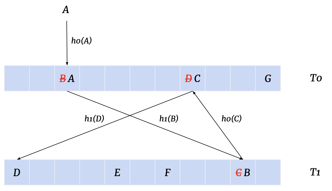
To keep memory in check, IDs seen only a few times aren't admitted at all, and IDs inactive for a set period expire. One more trade from the paper sticks in the mind: training servers are snapshotted only once a day. With a 0.01% daily failure rate per server, losing a day's updates on one server out of a thousand every ten days was judged harmless, and it saved a lot of copying.
08Features, and the gap between training and serving
8.1Training-serving skew
The ranker in section 6 runs on features of the pair, Ana and a title. Those features have to be computed twice: once offline, for every historical example the model trains on, and once online, at the moment Ana opens the app. If the two computations disagree, even slightly, the model is being served inputs unlike the ones it learned from. This mismatch is called training-serving skew, and it's one of the most common ways a recommender quietly gets worse.
It creeps in easily. Perhaps the offline version reads a warehouse table that's a day behind; the online one calls a live service. One rounds timestamps to the day, the other doesn't. Or, worst of all, the offline version accidentally uses information from after the moment being predicted: "number of times Ana watched this title" computed over all of history includes the very play the model is meant to predict. That's called leakage, and it makes a model look brilliant offline and useless online.
Martin Zinkevich's widely read "Rules of Machine Learning" from Google gives the simplest fix as Rule 29: "The best way to make sure that you train like you serve is to save the set of features used at serving time", and log them for training. It adds that the YouTube home page "switched to logging features at serving time with significant quality improvements". Its cost: a new feature can only be evaluated after it has been deployed and logged for weeks.
8.2Netflix's time machine
Netflix described a middle path in 2016, in a post titled "Distributed Time Travel for Feature Generation". Its researchers wanted three things at once: try a new feature on historical data without deploying it, compute it with exactly the code used online, and never let the future leak into the past ("no paradoxes", as the post puts it, "the label can't be in the features").
Netflix's answer was a time machine. Every day, a job picks a sample of contexts, member profiles with their devices and times, and snapshots what Netflix's online services returned for them: viewing history, My List, predicted ratings and so on, stored as Parquet files in S3. A system called DeLorean then takes an experiment's list of (context, time, title, label) examples, fetches the snapshots for each time, and runs the same feature encoders, the functions that turn raw data into features, that the online service runs. The features for a training example are computed from what the services knew at that moment, by the code that will compute them in production.
Streaming systems do the same thing continuously. Monolith's online joiner, from section 7.2, pairs each user action with the features that were served for that request, matched by a unique request key, and keeps features on disk for actions that arrive days later. That's "log features at serving time", done as a stream.
A feature store is the general name for the system this grows into: one place that defines each feature once, computes it for training with point-in-time correctness and serves it online with low latency. Uber described one in its 2017 post on its Michelangelo machine-learning platform, and the problem it solves is exactly the one in Netflix's 2016 post.
How should training features be produced?
- Try new features instantly
- No production changes
- Two implementations that drift apart
- Easy to leak the future
- No skew by construction
- A new feature must be deployed and logged for weeks before it can be tested
- One implementation
- New features testable on the past
- Point-in-time correct
- Snapshots cost storage
- Only sampled contexts are covered
Netflix chose the time machine in 2016 because its researchers needed to iterate on features quickly without each idea becoming a production project. The post also notes it stores a confidence level per snapshot, the fraction of service calls that succeeded without falling back, so an experiment can tell whether its historical inputs are trustworthy.
09Building the page from rows
9.1Why rows?
We can now rank titles for Ana. But her screen is a grid of rows, not a single list. Netflix's 2015 post on page generation, by Chris Alvino and Justin Basilico, explains why. A page of coherent, named rows lets a member decide about a whole group at a glance: scroll down past Comedies tonight, or right along Scandinavian Thrillers to see more. That lets the page be diverse without being confusing. Each row can be tightly focused, and the variety comes from having different rows, so the page serves tonight's mood, Ana's other moods, and the other people who share the account.
As the post describes it, the pipeline has five steps. Generate candidate rows likely to be relevant for this member, each with its evidence, such as the titles she watched in that genre. Filter each row's titles, for maturity rating or because she's already watched them. Rank the titles within each row with a row-appropriate ranker. Select and order rows to fill the page. Finally deduplicate titles across rows and fit rows to the device's limits.
The 2015 paper lists the rankers behind the main row types: the personalised video ranker for genre rows, a Top-N ranker tuned only for the head of the list for Top Picks, a trending ranker that picks up both yearly patterns like romance around Valentine's Day and one-off events like a hurricane in the news, a Continue Watching ranker that guesses whether you mean to resume, rewatch or have abandoned something, and sims for Because You Watched.
9.2Choosing rows: template, ranking, greedy
For a long time Netflix built pages from a template: fixed rules saying which kind of row goes in which position for every member, such as Continue Watching first, then Top Picks, then Popular, then five genre rows. Only the choice of rows within each type was personalised. It was tuned with A/B tests, but the rules grew complex and ignored things like a row's quality or the page's diversity. According to the 2015 paper, Netflix used it until 2015.
A next idea is to score each row on its own and sort, called row ranking. It's fast, but it has no idea of diversity, so a page can fill up with late-night comedies, family comedies, romantic comedies and action comedies. The fix the post describes is stage-wise selection: choose the best row for slot 1, then re-score every remaining row for slot 2 taking into account the rows and titles already chosen, and so on. Here is that greedy process on a few of Ana's candidate rows:
Greedy selection isn't guaranteed to find the best page: a good choice for slot 2 can leave nothing good for slot 9. Looking a few rows ahead helps at extra cost, and the ultimate version, scoring whole pages, is the integer-programming problem with the astronomically many pages from section 1. Netflix's 2015 paper describes its algorithm at the time as "fully personalized and mathematical", selecting and ordering rows from a large pool without a template, free to give one member no Because You Watched row at all and another half a page of them. Its exact algorithm is unpublished.
?Does it matter which corner a title is in?
Very much. The 2015 post notes that members scan down more than across, so titles near the top left are far more likely to be seen than those at the bottom right. That matters twice. When building the page, the most relevant titles belong where eyes go first. And when learning from the page, a title that wasn't played because it sat far off to the right tells you little about whether Ana would have liked it. This is position bias, and section 12 shows how Netflix's experiments correct for it.
Rows and pages are scored by a function that is itself learned. The 2015 post lists the kinds of features: the titles in the row and how well each is predicted to suit the member, the strength of the row's evidence, the member's past interactions with this row or similar ones, how long the row is, where it would sit, and how often it's been shown before.
10Choosing the picture for each title
10.1One image, chosen per member
The last decision on Ana's page is the one she noticed first: the picture. Netflix's December 2017 post on artwork personalisation explains why it matters. The image is evidence for why a title might suit her, especially for a title she's never heard of. Its example is Good Will Hunting: someone who watches many romantic films might be drawn by an image of Matt Damon and Minnie Driver, someone who watches comedies by one of Robin Williams. Netflix had earlier used bandit algorithms to find the single best image per title for everyone; the 2017 work personalised it per member.
It's harder than ranking titles, for a reason the post spells out. A row shows many titles and the member's choice among them is informative. But each title gets exactly one image, so if Ana plays the film, it was with the image she was shown; nobody knows what she'd have done with another. And the scale is large: the post says the system handles a peak of over 20 million requests a second, choosing from up to a few dozen candidate images per title.
10.2Exploration versus exploitation
Picture a row of slot machines, each paying out at a different, unknown rate. You can keep pulling the one that has paid best so far, which is exploitation, or try others in case one is better, which is exploration. Pull only the best-so-far and you may never discover a better machine; explore too much and you waste pulls on bad ones. This is the multi-armed bandit problem, named after the "one-armed bandit" slot machine, and choosing an image is one: each impression is a pull, a play is a payout.
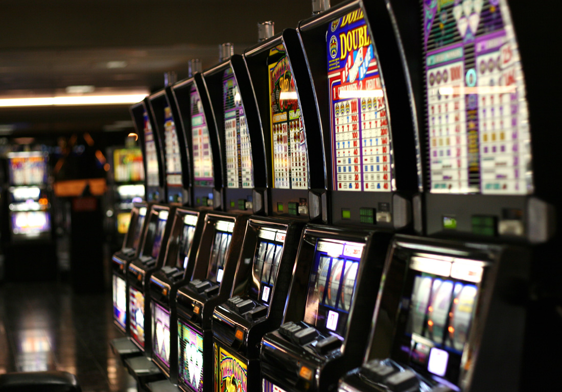
When the best machine depends on who's pulling, the problem becomes a contextual bandit: the context, here the member, their history, country, language, device and time, is an input, and the algorithm learns which image works best for each context. Netflix's post describes exploration by injecting controlled randomness into the model's choices, from simple epsilon-greedy (with some small probability, show a random image instead of the predicted best) to schemes that explore more where the model is less certain.
This program simulates the difference. A title has three images. Comedy fans, 60% of viewers, play it most with the comedian on it; romance fans with the couple. Each policy explores 10% of the time and otherwise shows the image with the best observed take rate, either for everyone or separately per kind of viewer:
import random
random.seed(11)

images = ["couple", "comedian", "skyline"]
# chance that one impression leads to a play, by kind of viewer (made up)
take = {"comedy fan":  {"couple": 0.02, "comedian": 0.06, "skyline": 0.03},
        "romance fan": {"couple": 0.07, "comedian": 0.02, "skyline": 0.03}}

def run(policy, n=200_000, eps=0.1):
    shows = {}; plays = {}; total = 0
    for _ in range(n):
        viewer = "comedy fan" if random.random() < 0.6 else "romance fan"
        ctx = viewer if policy == "contextual" else "everyone"
        if policy == "random" or random.random() < eps:
            img = random.choice(images)                     # explore
        else:                                               # exploit
            img = max(images, key=lambda i: plays.get((ctx, i), 0) /
                      max(1, shows.get((ctx, i), 0)))
        played = random.random() < take[viewer][img]
        shows[ctx, img] = shows.get((ctx, img), 0) + 1
        plays[ctx, img] = plays.get((ctx, img), 0) + played
        total += played
    return total / n * 1000

best = 0.6 * 0.06 + 0.4 * 0.07
print(f"random image:           {run('random'):.1f} plays per 1,000 impressions")
print(f"one best image for all: {run('bandit'):.1f}")
print(f"best image per viewer:  {run('contextual'):.1f}")
print(f"perfect knowledge: {best * 1000:.1f}")random image: 37.8 plays per 1,000 impressions
one best image for all: 43.1
best image per viewer: 61.7
perfect knowledge: 64.0The non-contextual bandit finds the comedian image, the best single choice, and improves on random by about 14%. Its contextual cousin learns a different image for each kind of viewer and gets within 4% of perfect knowledge. That remaining gap is the price of exploring: one impression in ten still goes to a random image. These take rates are invented, but the shape matches what Netflix reported: in offline evaluation, contextual bandits beat both random selection and the single-best-image bandit, and an A/B test showed "a significant lift in our core metrics". Lift was largest for titles the member had never interacted with, which makes sense, since the picture matters most when the title is unfamiliar.
The post explains why exploration is affordable at Netflix's size: spread over a hundred million members, each member only helps explore images for a small part of the catalogue, so the cost per member is negligible. It also guards against two traps. Images that tempt a play but lead to poor viewing are clickbait, so the label is a quality play, not any play. And images aren't swapped too often for the same member, both so Ana can still recognise a title she noticed yesterday and so each play can be credited to one image.
10.3Evaluating a policy without running it
How do you test a new image-selection model before showing it to anyone? Netflix's post describes replay. During exploration, some images were shown at random, and the system logged which image was shown with what probability, and whether a play followed. To evaluate a new model, go through the randomly chosen impressions and keep only those where the random choice happened to match what the new model would have chosen; the take rate on that subset is an unbiased estimate of how the new model would perform. Netflix reported a reasonable correlation between replay results and the online A/B test.
11Feedback loops
11.1The system trains on its own output
Everything the system learns comes from what members did with the pages it showed them. That creates a loop: the model shows Ana crime dramas, she watches crime dramas because that's what's in front of her, and the training data says she likes crime dramas even more. Titles never shown never get plays, so the model never learns they were good. Left alone, the loop narrows what each member sees and concentrates viewing on titles that were popular to begin with. When the narrowing reaches a member's whole view of the world, as in news or social media, it's often called a filter bubble.
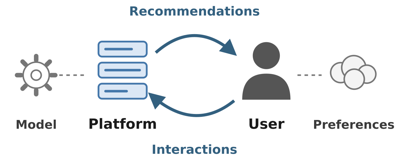
Several designs we've already met push back against the loop. Exploration (section 10) deliberately shows some things the model isn't sure about. Page diversity (section 9) gives other tastes some rows. YouTube's 2016 paper adds one more: it trains on all watches, including those that came from search or links on other sites, not only on watches of its own recommendations, because otherwise "it would be very difficult for new content to surface and the recommender would be overly biased towards exploitation". And TikTok's 2020 explanation of its For You feed acknowledges that optimising for relevance risks an ever more uniform stream of videos, and says the feed generally won't show two videos in a row by the same creator or with the same sound.
11.2Measuring spread: effective catalogue size
Netflix's 2015 paper measures how concentrated viewing is with a metric it calls effective catalogue size (ECS): close to 1 if almost all viewing goes to a single title, close to the number of titles if viewing is spread evenly. Comparing viewing under personalised ranking with an unpersonalised popularity ranking, it found the effective catalogue size roughly four times larger with personalisation, at the median rank of the titles people played. In other words, at Netflix's scale personalisation spread viewing across more of the catalogue than a single "most popular" list would have, which is the opposite of the bubble. That doesn't make the loop go away; it means the loop has to be watched with a metric, not argued about.
12How Netflix knows a change worked
12.1A/B tests on retention
Offline metrics guide development, but every source in this chapter says the same thing about them: they don't reliably predict what happens with real members. YouTube's paper says live A/B results "are not always correlated with offline experiments". Netflix's 2015 paper gives an example where intuition failed too: of two lists of titles similar to House of Cards, the one that looked less relevant to people did better in a test, because it leaned more on popular titles.
So the final judge is an A/B test, a randomised controlled experiment: members are assigned at random to groups Netflix calls cells, one getting the current experience (the control) and others the new algorithms. Netflix's 2015 paper describes letting members use the product for typically two to six months, then comparing streaming hours and, above all, retention between cells. Each member keeps the same experience for the whole test, which costs statistical power compared with randomising per session, but is the only way to see effects on overall engagement and cancellation over many sessions.
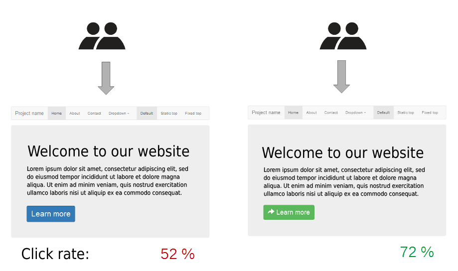
The difficulty is sensitivity. Netflix's retention is already high, so even a 0.1% change in retention takes a very meaningful improvement. The 2015 paper describes three levels of win: a local win, where members engage more with the part that changed; an overall engagement win; and a retention win. It reports finding multiple clear retention wins every year, but many more local wins that don't move the totals, often because the changed row takes viewing from other rows.
12.2Interleaving: a faster first round
Tests that need months and large groups limit how many ideas can be tried. Netflix's November 2017 post describes a two-stage process: a fast first stage to prune many ranking ideas down to a few promising ones, then ordinary A/B tests on the survivors.
The first stage uses interleaving. Instead of showing group A ranker A's row and group B ranker B's, every member in the test gets one row blended from both, and the comparison is which ranker's titles they watch more of. It works like a blind taste test where each person gets both drinks: differences between heavy and light viewers cancel out, because each member is compared with themselves.
The blending has to respect position bias, since titles on the left get played more regardless of quality. Netflix uses a variant of team-draft interleaving, named after picking teams for a match: a coin toss decides which ranker picks first, then they take turns, each adding its highest-ranked title not already chosen. Every position is equally likely to come from either ranker, and each title's viewing hours are credited to the ranker that contributed it.
Netflix reported a large payoff. Comparing two rankers of known relative quality, interleaving needed more than 100 times fewer members than the most sensitive A/B metric to pick the better one with 95% reliability, and the first stage finishes in a matter of days.
How should ranking changes be tested?
- Instant and free
- Many ideas per day
- Often disagrees with live results
- Biased by the old model's choices
- Measures what the business cares about
- Needs large cells and months per test
- Few ideas tested per year
- Many ideas tried quickly
- Final decision on retention
- Interleaving only works for comparing rankings
- More experiment machinery to build
Netflix described this two-stage online process in 2017 with offline evaluation before it, and replay for bandits (section 10.3) fills the same role for policies that can't be interleaved. What's being optimised hasn't changed since 2015: medium-term engagement and retention, measured in A/B tests.
13One model for many rows
13.1Netflix's foundation model (2025)
By the 2020s, the design so far had produced many specialised models, one for Continue Watching, one for Top Picks, and many more, each trained separately on overlapping data. Netflix's March 2025 post describes the cost of that: maintenance became expensive, and an improvement in one model was hard to carry over to the others. Many of the models also looked only at a short window of recent history, because of latency and training cost.
Its answer borrows from large language models. A single large foundation model is trained on members' full interaction histories, treated as sequences of tokens, much as a language model treats text. Netflix described "hundreds of billions" of interactions from its 300 million members. Raw events are merged into meaningful tokens, for example combining several plays of the same title into one with the total watch time, a trade-off between keeping detail and keeping sequences short. The model learns to predict the next interaction, with some changes for recommendations: not every event counts equally (a five-minute trailer isn't a two-hour film), it predicts several future items to avoid being short-sighted, and it predicts auxiliary targets like genre too.
Netflix's post is open about the serving constraint. Recommendation services answer in milliseconds, so at inference time the context is limited to hundreds of events, not the thousands an active member generates. Other systems use the foundation model in three ways: directly, through its prediction heads; by fine-tuning it for a specific part of the product; or through its embeddings, computed in batch and used as features or for candidate generation. Because each retraining would scramble the meaning of the embedding dimensions, Netflix applies a transformation that keeps the space stable across versions, so downstream models don't break.
14The whole system
14.1Every box, and why it's there
| Component | What it does | Added because |
|---|---|---|
| Embeddings (two towers, foundation model) | A vector for every member and title | Taste must be compared cheaply; new titles need a vector on day one (§3, §13) |
| Candidate generation and ANN index | Cuts the catalogue and row pool to hundreds | The heavy model can't score everything (§4, §5) |
| Rankers | Order titles in each row by a proxy for satisfaction | Plays alone reward clickbait (§6) |
| Offline / nearline / online split | Puts each computation where its staleness is acceptable | Fresh results without request-time cost (§7) |
| Feature store and time machine | Same feature code for training and serving | Training-serving skew and leakage (§8) |
| Page builder | Chooses and orders rows | One ranked list isn't a usable page (§9) |
| Artwork bandit | Picks an image per title per member | The image is evidence, and only one can be shown (§10) |
| Exploration and diversity | Shows some uncertain or different things | The loop trains on its own output (§11) |
| Experimentation | Interleaving, then A/B tests on retention | Offline metrics mislead (§12) |
14.2From top to bottom
| Level | The choice | Data structure or algorithm |
|---|---|---|
| System | Decompose the page: titles, rows, page, images | Funnel: candidate generation → ranking → page assembly |
| Representation | Members and titles as vectors | Matrix factorisation; two-tower networks; transformer over interaction tokens |
| Retrieval | Nearest vectors, approximately | IVF lists from k-means; product-quantised codes; HNSW layered graphs |
| Ranking | Predict a satisfaction proxy | Neural networks over hundreds of features; weighted sum of predicted outcomes |
| Freshness | Offline, nearline, online | Batch jobs; event-driven updates; minute-level embedding sync (Monolith) |
| Embedding tables | No two IDs share a vector | Cuckoo hash table with frequency filtering and expiry (Monolith) |
| Features | Point-in-time correctness | Daily snapshots of service data replayed through shared feature encoders |
| Page | Relevance plus diversity | Greedy stage-wise row selection with a diversity penalty |
| Artwork | Learn while serving | Contextual bandit with epsilon-greedy or uncertainty-driven exploration; replay evaluation |
| Measurement | Sensitive first, decisive second | Team-draft interleaving; A/B cells judged by retention |
15What goes wrong, and the tradeoffs
15.1Failures this design has to survive
| What happens | What the member sees | What the design does |
|---|---|---|
| A request-time model is slow or down | A page that's a little less personal | Online services fall back to precomputed lists |
| A new title launches with no plays | It still appears for likely fans | Metadata-based embeddings; image exploration from day one |
| A feature is computed differently in training | Recommendations quietly get worse | One feature-encoder library, time-machine snapshots, logged serving features |
| The model learns from its own choices | A narrowing page | Exploration, diversity in page building, training on non-recommended viewing |
| An image wins plays but disappoints | Clickbait artwork | Labels count quality plays, not any play |
| An offline win loses online | Wasted launch effort | Interleaving and A/B tests decide; misalignment prompts a reward fix |
| The household shares one profile | A muddled page | Diverse rows cover several tastes at once |
15.2The tradeoffs, in one table
| Decision | Chosen | Given up | Why it was worth it |
|---|---|---|---|
| Prize ensemble | Two simpler models from the 2007 progress prize | The last few percent of accuracy | Engineering cost outweighed the accuracy gain |
| Target | Engineered satisfaction proxy | Simple, observable labels | Plays alone reward clickbait; retention is too slow |
| Where to compute | Mix of offline, nearline, online | One simple system | Freshness where it matters, cost where it doesn't |
| Retrieval | Approximate nearest neighbours (at scale) | A few true neighbours | Orders of magnitude less work per query |
| Training features | Time-machine replay of production code | Storage for snapshots | No skew, and new features testable on history |
| Page layout | Learned row selection (since 2015) | The simplicity of a template | Diversity and per-member page shape |
| Artwork | Contextual bandit with exploration | A small exploration cost per member | Much better image choices, learned continuously |
| Testing | Interleaving, then A/B | Some experiment complexity | Over 100 times more sensitive first stage |
16Summary
- A home page is many decisions: which rows, which titles in each, in what order, with which image, for one member on one device, from tens of thousands of candidate rows.
- Predicting stars was the wrong target: the Netflix Prize's winning ensemble was never shipped, and streaming made plays, completions and abandonment far more informative than ratings.
- Matrix factorisation learns a vector for every member and title, and the dot product of two vectors predicts how well they match; these vectors are embeddings.
- Two-tower models compute embeddings from features, so new titles get vectors from metadata, and title vectors can be computed ahead of time.
- The system is a funnel because a rich model can't score everything: cheap retrieval to hundreds, heavy ranking, then page assembly.
- Approximate nearest-neighbour indexes trade a little recall for a lot of speed: inverted files scan a few k-means clusters, product quantisation compresses vectors, and HNSW walks layered graphs like a skip list.
- The ranker should predict a proxy for long-term satisfaction, not just plays, with delayed feedback predicted so training stays fresh.
- Each computation runs offline, nearline or online according to how stale it can afford to be, with precomputed fallbacks.
- Training and serving must compute features the same way; Netflix's time machine replays daily snapshots through the production feature code.
- Pages are built row by row, greedily trading relevance against diversity, and the picture on each title is chosen by a contextual bandit that keeps exploring.
- Offline metrics mislead, so experiments decide: interleaving prunes ideas in days, and A/B tests on retention make the final call.
17Build this
A small home-page builder.
- Download the MovieLens 25M dataset (public, from GroupLens). Treat ratings of 4 and above as plays. Hold out each user's last few plays by time.
- Train a matrix factorisation with 32 numbers per vector. Measure how often a user's held-out plays appear in their top 100 by dot product (recall at 100).
- Put the movie vectors in an HNSW index (the
hnswlibpackage) and in a Faiss IVF index. Compare recall and query time against an exact scan as you varyefandnprobe. - Build rows from genres and from "because you watched" neighbours. Assemble a 10-row page greedily, with a penalty for overlap between rows, and compare the number of distinct genres on the page with and without the penalty.
- Simulate artwork: invent three images per movie with take rates that depend on the user's favourite genre, and compare a single-best-image bandit with a contextual one, as in section 10.
- Finally, implement team-draft interleaving between two of your rankers on simulated users, and count how many users each method needs to pick the better ranker reliably.
18Interview questions
beginnerWhy didn't Netflix use the algorithm that won the Netflix Prize?›
The winning entry blended hundreds of models to beat Cinematch's error by 10%. Netflix had already put the two strongest components from the first progress prize, a matrix factorisation and a restricted Boltzmann machine, into production after scaling them from 100 million to 5 billion ratings. Its engineers judged that the extra accuracy of the full ensemble didn't justify the engineering cost of running it, and by then streaming had moved the focus from predicting stars to the whole page.
beginnerWhat is an embedding, and how is it used to recommend?›
An embedding is a vector of numbers learned for each member and each title, arranged so that a member's vector points in a similar direction to the vectors of titles they enjoy. A recommendation then becomes a geometric question: which title vectors are closest to this member's vector, by dot product or cosine similarity. Titles similar to a given title are its nearest neighbours in the same space.
intermediateWhy is a recommender built as a funnel of candidate generation, ranking and re-ranking?›
The best predictions come from models with hundreds of features of the member and title together, and running one on every item for every request costs too much: a modest three-layer network is millions of operations per item. So a cheap stage, usually nearest-neighbour search over embeddings plus rules, picks a few hundred candidates; the heavy model ranks only those; and a final stage applies page-level concerns like diversity and filtering. YouTube described this in 2016 as millions of videos to hundreds to dozens.
intermediateCompare IVF and HNSW indexes for nearest-neighbour search.›
IVF clusters the vectors with k-means and stores each cluster as a list; a query compares itself with the cluster centres and scans only the nearest few lists, controlled by nprobe. Combined with product quantisation it stores vectors in tens of bytes, so it scales to billions. HNSW links each vector to its near neighbours in a stack of graphs, sparse at the top like a skip list, and searches greedily from the top layer down; it gives high recall at low latency and easy insertion, but costs memory for the links. Both trade recall for speed with one parameter (nprobe, ef). For a catalogue of thousands, an exact scan is simpler.
deepWhat is training-serving skew, and how would you prevent it?›
It's when the features a model is trained on are computed differently from the ones it's served, so live inputs don't look like training inputs. Causes include two implementations of the same feature, different data freshness, and leakage of information from after the prediction time. Fixes: log the features the model was served and train on the log; or, as Netflix did in 2016, snapshot online service data daily and replay it through the same feature-encoder code for any past time; and in general use a feature store that defines each feature once with point-in-time correctness.
deepHow would you choose which image to show for each title, and how would you evaluate a new policy?›
Treat it as a contextual bandit: each impression picks one image given the member's context, and a quality play is the reward. Explore with controlled randomness, from epsilon-greedy to uncertainty-driven schemes, and log the probability of each choice. Label quality plays, not any play, to avoid clickbait, and don't change a member's image too often. To evaluate a new policy offline, replay the logged random impressions, keeping only those where the random choice matches the new policy's, and measure the take rate there; then confirm with an A/B test. Netflix did this in 2017 and found the largest lift for titles the member didn't already know.
deepWhy does Netflix use interleaving before A/B testing?›
Retention, the metric that matters, moves slowly and only for members near cancelling, so A/B tests need large cells and months. Interleaving blends two rankers' results into one row for each member, using team-draft picks so each position is equally likely to come from either, and credits viewing to the ranker that contributed each title. Since each member is compared with themselves, the noise from heavy and light viewers cancels, and Netflix found it needed over 100 times fewer members than its most sensitive A/B metric. It's used to prune ideas in days, with A/B tests on the survivors.
19Go deeper
An IVF index with nprobe = 1 returns only about half the true nearest neighbours. Why, and what do you change?›
Many queries sit near the edge of their cluster, so some true neighbours are in the adjacent clusters, which nprobe = 1 never scans. Raise nprobe (search more lists), at the cost of more distance computations; in the TryIt, nprobe = 16 reached 99% recall for a sixth of the scan's work.
Why does a contextual artwork bandit still lose a little to perfect knowledge, even after it has learned which image is best?›
Because it keeps exploring: some fraction of impressions still go to an image chosen at random, to keep learning as titles and tastes change. That small, ongoing cost is the regret of exploration, spread thinly across many members.
Your new ranker beats the old one offline but loses the A/B test. Name two likely causes.›
The offline data was logged under the old model, so it rewards agreeing with it; or the offline target (the proxy reward) isn't aligned with what the A/B test measures. Training-serving skew in the new model's features is a third.
The algorithms behind each row, page generation, evidence, effective catalogue size, the business value, and how Netflix runs A/B tests.
The prize and its aftermath, and the offline, nearline and online architecture.
Row selection, diversity and navigation; contextual bandits for images, exploration and replay.
Feature generation without skew, faster experiments, reward engineering, and one large model shared by many rows.
The funnel, candidate generation as classification, nearest-neighbour serving, and weighted logistic regression for watch time.
The layered graph index, and the inverted-file and product-quantisation toolkit with its trade-offs.
Collisionless embedding tables on cuckoo hashing, and online training with minute-level parameter sync.
An open-sourced production recommender: candidate sources, a 48-million parameter ranker, and its published engagement weights.
20Related chapters
Another index for "what's near this point", in two dimensions instead of hundreds. Chapter 50.
The event streams that carry plays and impressions to nearline and offline jobs. Chapter 23.
Precomputed results served from caches like EVCache, and what staleness they allow. Chapter 25.
The Parquet files and warehouse queries behind offline training data. Chapter 24.
Monitoring models and features in production, where quiet degradation is the usual failure. Chapter 39.