Here are eight orders from a small shop, one row each. Every row says when the order happened (ts, in seconds, with one order every three seconds), which user placed it, which country they live in, and how much they spent.
| ts | user_id | country | amount |
|---|---|---|---|
| 0 | 41 | US | 10 |
| 3 | 7 | IN | 5 |
| 6 | 93 | US | 20 |
| 9 | 18 | DE | 7 |
| 12 | 66 | IN | 8 |
| 15 | 12 | US | 30 |
| 18 | 85 | DE | 3 |
| 21 | 30 | IN | 12 |
Someone asks for the total amount per country. On eight rows you'd do it by eye: US 60, IN 25, DE 10. Real tables hold millions or billions of rows, the question stays the same, and the way the table is laid out on disk decides whether the answer takes a few milliseconds or a few seconds.
Look at what the question needs from each row. It needs country and amount, and nothing else. Think of a paper filing cabinet where every order has its own folder holding all four facts. To total the amounts you'd open every folder and copy out two numbers, carrying the other two facts along each time. File the same information the other way, one long sheet holding all the amounts and another holding all the countries, and you read two sheets straight down.
Databases that file by folder are the ones you probably know, and engines built for analysis file by sheet. The question this chapter answers is how a query over ten million rows can finish in a few milliseconds. The sheet layout is where the answer starts, and it leads to four tricks that stack: read only the sheets you need, shrink each sheet, skip parts of a sheet before reading them, and process the values in batches the CPU likes. We'll time the gap on a real file first, then take the eight rows apart one trick at a time, and finish with three real systems that put the tricks to work.
01Timing one query on two files
1.1Ten million rows, one query
Before we take anything apart, let's measure the gap on a real file. The script below needs Python and DuckDB (pip install duckdb). DuckDB is a database that runs inside your Python process like a library and can query files directly; section 9 comes back to it.
The script writes a table of ten million rows twice. One copy is a CSV file, a plain text file with one row per line and the values separated by commas, so it stores the table row by row. The other is a Parquet file, a format that stores the table column by column. Then the script asks each file the same question as our eight rows, the total amount per country. The data is synthetic, generated by the script itself.
A few lines need explaining. range(10000000) produces the numbers 0 to 9,999,999, and each number becomes one row. The ARRAY[...] expression picks one of eight country codes from the row number by arithmetic. COPY (query) TO 'file' writes the result of a query into a file, and the option in brackets chooses the format. Each timed query runs twice. The operating system keeps recently read files in memory, so the first run loads the file into that cache and the second, timed run measures the engine and not the disk. fetchall() pulls the result rows into Python, which forces the query to finish before the clock stops.
import os, time, duckdb

con = duckdb.connect()
con.execute("""
    COPY (SELECT i AS user_id,
                 (ARRAY['US','IN','DE','BR','JP','GB','FR','CA'])[1 + (i * 7919 % 8)] AS country,
                 round((i * 31 % 10000) / 100.0, 2) AS amount
          FROM range(10000000) t(i))
    TO 'events.csv' (HEADER, DELIMITER ',')""")
con.execute("COPY (SELECT * FROM 'events.csv') TO 'events.parquet' (FORMAT PARQUET)")
print(f"CSV     : {os.path.getsize('events.csv') / 1e6:7.1f} MB")
print(f"Parquet : {os.path.getsize('events.parquet') / 1e6:7.1f} MB\n")

q = "SELECT country, sum(amount) FROM '{}' GROUP BY country ORDER BY country"
for name in ("events.csv", "events.parquet"):
    con.execute(q.format(name)).fetchall()                 # warm the file cache
    t = time.perf_counter()
    con.execute(q.format(name)).fetchall()
print(f"GROUP BY over {name:<15}: {(time.perf_counter() - t) * 1000:8.1f} ms")CSV : 166.9 MB
Parquet : 63.3 MB
GROUP BY over events.csv : 127.6 ms
GROUP BY over events.parquet : 6.1 msTwo numbers stand out. The Parquet file is about 2.6 times smaller than the CSV, 63.3 MB against 166.9 MB, and the same query runs about 21 times faster on it, 6.1 ms against 127.6 ms. Timings change from machine to machine, but a gap of this shape shows up everywhere.
1.2Where the gap comes from
The query uses two of the file's three columns, country and amount. A CSV has no way to jump to them: it has to read and parse every byte of every row to find them. Parquet keeps each column together, so the engine reads only the two columns it needs, and each of them is stored in an encoded form that is much smaller than its text.
Those are the first two of the four tricks. The other two are skipping chunks of a column before reading them, using statistics stored in the file, and processing the values in batches sized for the CPU. This data is synthetic and very regular, so the encodings do unusually well on it, and real tables usually compress less.
To see each trick working, we need something we can hold in our heads. So we shrink the table back to the eight orders from the opening and ask how they would be stored.
02Two ways to lay out a table
2.1The eight orders, stored two ways
A table is a grid, but a file is one long line of bytes, so the first decision a database makes is the order in which the grid's values go into that line. One order goes row by row: all four values of the first order, then all four of the second, and so on. This is the row layout. The other goes column by column: all eight ts values, then all eight user_id values, then the countries, then the amounts. This is the column layout. A database built around the first is a row store (Postgres, MySQL and SQLite are row stores), and one built around the second is a column store.
The order matters because storage hands data over in fixed-size chunks called blocks, a few kilobytes each, and memory moves data between its levels in similar small chunks. Asking for one number brings its whole block along, with whatever sits next to it. Here are our eight orders written both ways, followed by the work our query has to do on each:
?Why can't the row layout just skip the values it doesn't need?
Because its values are bundled by row, and storage reads whole blocks. The amount of row 1 shares a block with the ts, user_id and country of row 1 and with the neighbouring rows, so there is no block that holds amounts and nothing else. A query that wants one value per row pays for all of them. For a query that scans millions of rows that's a bad deal. For a query that wants one whole row, it's exactly right, because the whole row arrives in one block. So which layout wins depends on which kind of query you run most.
2.2Two workloads, two layouts
The two kinds of query have names. Systems that handle orders, accounts and messages one record at a time run transactional workloads, abbreviated OLTP for "online transaction processing". Systems that answer questions about a whole table, like ours, run analytical workloads, abbreviated OLAP for "online analytical processing". The two want opposite things.
| Transactional (OLTP) | Analytical (OLAP) | |
|---|---|---|
| Typical query | Fetch or update one order by id | Sum revenue by country for a quarter |
| Rows touched | A handful | Millions to billions |
| Columns touched | Most of them | Two or three out of dozens |
| Writes | Constant, small, in place | Bulk appends, rarely updates |
| Layout that fits | Row store: Postgres, MySQL, SQLite | Column store: Parquet, ClickHouse, DuckDB |
A row store keeps each row's values next to each other, so fetching order 42 is one block read. A column store keeps each column's values next to each other, so summing one column reads only that column's blocks. Our question is analytical, and so is every measurement in the rest of the chapter.
2.3The table the chapter measures
From here on, the real measurements all use one synthetic table of 10 million events, generated inside DuckDB. It is our eight-row table grown up, with two more columns (event_type and url), and with the same one-event-every-three-seconds clock.
| Column | Type | Shape |
|---|---|---|
ts | timestamp | Increasing, one event every 3 seconds through 2026 |
user_id | int32 | Pseudo-random, about 1 million distinct values |
country | string | 10 distinct values |
event_type | string | 4 distinct values |
amount | double | Pseudo-random, 0 to 999.99 |
url | string | https://shop.example/p/ plus one of 5 million ids |
As CSV the table is 725 MB, roughly 72 bytes a row. Loaded into SQLite, a row-store database that keeps everything in one file, it is an 804 MB file. Written to Parquet with pyarrow's defaults (pyarrow is Python's Apache Arrow library, which can write Parquet) it is 224 MB.
Now think about SELECT sum(amount). The row store has to read its whole file. The Parquet file has a separate stretch of bytes for amount, and the engine reads only that:
| Bytes a row store must read | the whole SQLite file | 804 MB |
| Bytes the amount column occupies in Parquet | sum of its column chunks | 26 MB |
| Ratio | 804 / 26 | ≈ 31× |
| Less data to read for the columnar layout | ≈ 31× | |
Part of that 31 comes from the layout and part from the way Parquet writes each column smaller than its text, which section 4 takes apart.
2.4What a column store buys on one query
Let's see what the layout is worth in time. The same data was loaded into SQLite and into DuckDB's own file format, with a warm cache, and each number is the median of three to five runs. DuckDB can use several threads, which are separate streams of work running on separate CPU cores, so the table shows one and four.
| Query | SQLite 3.53.3 | DuckDB table, 1 thread | DuckDB table, 4 threads |
|---|---|---|---|
| SELECT sum(amount) | 421 ms | 11.7 ms | 4.2 ms |
| SELECT country, sum(amount) GROUP BY country | 3,209 ms | 31.0 ms | 10.5 ms |
| File size on disk | 804 MB | 135 MB | 135 MB |
On one thread, DuckDB is 36 times faster on the sum and about 100 times faster on the group-by. The group-by gap is wider because of how each engine keeps its running totals. SQLite's plan for it is USE TEMP B-TREE FOR GROUP BY: it builds a B-tree (a sorted tree structure) keyed on country and inserts every row into it. DuckDB keeps ten running totals in a hash table, a structure that finds a value's slot directly from the value, so there is nothing to sort or rebalance.
That tells us the table compares two whole engines. The layout is part of the gap, and an engine built to chew through arrays of values is the rest, which we come to in section 6.
2.5What columns cost you
Columns aren't free. Each strength is a weakness for the other workload:
| Operation | Row store | Column store |
|---|---|---|
| Read a few columns of many rows | Reads every column | Reads only those columns |
| Fetch one whole row by key | One block | One separate read per column, then stitch the row back together |
| Insert one row | Append to one block | Touch every column's storage; engines buffer and batch instead |
| Update one field in place | Cheap | Usually a rewrite of a block, or a delete marker plus an insert |
| Compress | Mixed types side by side, so poorly | One type at a time, from about 2 times to about 900 times in the measurements of section 4 |
That's why the systems in this chapter all want data in big batches: Parquet writers buffer about a million rows before writing a group of rows, and ClickHouse turns every INSERT into a new immutable piece of storage (section 8). What we need now is a file format that holds column values in big batches and remembers where every batch is, so a reader can fetch one without reading the rest. Parquet is that format.
03Inside a Parquet file
Take the column layout literally and write the eight orders as four long arrays, one after another. For eight rows that works fine. For ten million it breaks three ways. The writer receives rows one at a time but has to write a column at a time, so it must hold the whole table in memory until the end. A reader that wants to use several CPU cores has only whole columns to hand out, one per core. And a reader that wants to skip the part of a column it doesn't need can't tell which part that is without reading it.
The fix is to cut the table into horizontal slices first and lay out each slice by column. That's the design of Parquet, the columnar file format most analytical tools read and write: Spark, Trino, DuckDB, ClickHouse, pandas, Polars, Snowflake's external tables. Its layout comes from Google's Dremel paper (VLDB 2010), and the format itself is defined in one file written in a notation called Thrift, which we'll look at in 3.3.
3.1Four levels: file, row group, column chunk, page
A Parquet file is a hierarchy. The horizontal slices are row groups. Inside a row group, each column's values for those rows are stored together as a column chunk. A chunk is cut into pages, the pieces that get encoded and compressed (section 4); a Parquet page has nothing to do with the memory pages of the operating system. At the very end of the file comes the footer, a block of metadata, meaning data about the data, that describes everything before it: the schema, and for every chunk its position in the file, its size, and the smallest and largest value it contains, called its min and max. Section 5 puts those min and max values to work.
| Level | What it holds | pyarrow default |
|---|---|---|
| File | The marker PAR1, the row groups, then the footer | |
| Row group | A horizontal slice of rows, stored column by column | up to 1,048,576 rows |
| Column chunk | One column's values for one row group, contiguous on disk | |
| Page | The piece a chunk is cut into, and the unit that gets compressed | about 1 MB, or 20,000 rows |
| Footer | Schema, and for every chunk its position, size, min and max | at the end of the file |
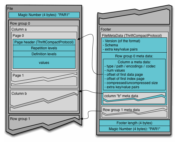
The row group answers the three problems from the start of the section. A writer has to buffer only one row group in memory before writing its columns one after another, so the group size caps the writer's memory. A row group is also the natural unit of parallel work, one core per group. And each group gets its own min and max per column, so a reader can rule out a whole group at a time.
?Why is the footer at the end?
Because the writer only knows the positions and statistics once it has written the data. Putting the metadata last lets it stream row groups out as they fill and write the index once, at the end. Readers pay for it: they have to start from the end of the file. The last 8 bytes hold the footer's length and the marker PAR1 again, so a reader fetches the tail, then the footer, then only the chunks it needs.
Here is that read path as a pipeline, for one column of one row group:
PAR1. On S3, Amazon's object storage, that's one ranged GET, a request for just those bytes.3.2Our eight orders as a Parquet file
Let's write our eight orders to a Parquet file and read the footer back. The script uses pyarrow. row_group_size=4 tells the writer to start a new row group after every four rows, so eight rows make two groups. ParquetFile(...).metadata reads the footer, and statistics on a column chunk gives its min and max.
import pyarrow as pa, pyarrow.parquet as pq

t = pa.table({
    "ts":      [0, 3, 6, 9, 12, 15, 18, 21],
    "user_id": [41, 7, 93, 18, 66, 12, 85, 30],
    "country": ["US", "IN", "US", "DE", "IN", "US", "DE", "IN"],
    "amount":  [10, 5, 20, 7, 8, 30, 3, 12],
})
pq.write_table(t, "toy.parquet", row_group_size=4)

m = pq.ParquetFile("toy.parquet").metadata
print(m.num_rows, "rows in", m.num_row_groups, "row groups")
for r in range(m.num_row_groups):
    for c in range(m.row_group(r).num_columns):
        cc = m.row_group(r).column(c)
print(r, cc.path_in_schema, cc.statistics.min, cc.statistics.max)8 rows in 2 row groups
0 ts 0 9
0 user_id 7 93
0 country DE US
0 amount 5 20
1 ts 12 21
1 user_id 12 85
1 country DE US
1 amount 3 30Each output line is a row group number, a column, and that chunk's min and max. Row group 0 holds the first four orders, whose ts runs from 0 to 9, and row group 1 holds the last four, with ts from 12 to 21. The two ts ranges don't overlap, because the orders were written in time order. The user_id ranges, 7 to 93 and 12 to 85, overlap almost completely, because the ids are scattered. Strings compare in alphabetical order, and both groups contain a DE and a US, so the two country ranges are identical. Keep these ranges in mind. They decide what can be skipped in section 5. First, where exactly does the format keep them? Its specification answers that.
3.3The footer, from the spec
Parquet's footer is described in a file written in Thrift, a notation for describing records so that programs in different languages can write and read the same bytes. Here is what the format's definition says each row group carries:
struct RowGroup {
  /** Metadata for each column chunk in this row group.
   * This list must have the same order as the SchemaElement list in FileMetaData.
   **/
  1: required list<ColumnChunk> columns

  /** Total byte size of all the uncompressed column data in this row group **/
  2: required i64 total_byte_size

  /** Number of rows in this row group **/
  3: required i64 num_rows

  /** If set, specifies a sort ordering of the rows in this RowGroup.
   * The sorting columns can be a subset of all the columns.
   */
  4: optional list<SortingColumn> sorting_columns
  /* ... file_offset, total_compressed_size, ordinal ... */
}
And for each column chunk:
struct ColumnMetaData {
  1: required Type type
  2: required list<Encoding> encodings
  3: required list<string> path_in_schema
  4: required CompressionCodec codec
  5: required i64 num_values
  6: required i64 total_uncompressed_size
  7: required i64 total_compressed_size
  /* ... */
  /** Byte offset from beginning of file to first data page **/
  9: required i64 data_page_offset
  /* ... */
  /** Byte offset from the beginning of file to first (only) dictionary page **/
  11: optional i64 dictionary_page_offset

  /** optional statistics for this column chunk */
  12: optional Statistics statistics;
  /* ... encoding_stats, bloom_filter_offset, bloom_filter_length, ... */
}
Field 12 is where skipping comes from. Statistics holds min_value, max_value and null_count, the number of missing values in the chunk, and the spec now asks readers to tell an absent null_count apart from zero. Fields 2, 4 and 11 matter for the next section: they record which encodings and which compressor the chunk uses, and where its dictionary page sits (the next section explains what a dictionary is).
3.4A real footer
Now the same thing at full size. To follow along, generate the 10-million-row table from 2.3 and write it with pyarrow's defaults, which means snappy compression (a fast compressor, covered in 4.5) and row groups of up to 1,048,576 rows. The generator below makes a table of the same shape. Its values are pseudo-random and its strings may differ from the original table's, so expect byte counts near the ones printed in this chapter but not on them. The timestamps and row groups come out exactly the same.
import duckdb, pyarrow.parquet as pq

con = duckdb.connect()
events = con.execute("""
    SELECT TIMESTAMP '2026-01-01' + to_seconds(3 * i)                          AS ts,
           (hash(i) % 1000000)::INTEGER                                        AS user_id,
           (ARRAY['US','IN','DE','BR','JP','GB','FR','CA','ES','NL'])
               [1 + (hash(i + 1) % 10)::INTEGER]                               AS country,
           (ARRAY['view','click','buy','refund'])[1 + (hash(i + 2) % 4)::INTEGER] AS event_type,
           round((hash(i + 3) % 100000) / 100.0, 2)                            AS amount,
           'https://shop.example/p/' || (hash(i + 4) % 5000000)                AS url
    FROM range(10000000) r(i)""").to_arrow_table()
pq.write_table(events, "events_snappy.parquet")
Reading the footer takes a few lines. The script prints the number of rows, the number of row groups and the footer's size in bytes, then each column's compressed size and min and max in the first row group, then the ts range of every row group.
import pyarrow.parquet as pq
m = pq.ParquetFile("events_snappy.parquet").metadata
print(m.num_rows, m.num_row_groups, m.serialized_size)

rg = m.row_group(0)
for c in range(rg.num_columns):
    cc = rg.column(c)
    s = cc.statistics
    print(cc.path_in_schema, cc.total_compressed_size, s.min, s.max)

for r in range(m.num_row_groups):          # the ts range of every row group
    s = m.row_group(r).column(0).statistics
print(r, m.row_group(r).num_rows, s.min, s.max)10000000 10 7940
ts 6755729 2026-01-01 00:00:00 2026-02-06 09:48:45
user_id 4688240 0 999997
country 529155 BR US
event_type 267050 buy view
amount 2702020 -0.0 999.99
url 8432088 https://shop.example/p/0 https://shop.example/p/999996
0 1048576 2026-01-01 00:00:00 2026-02-06 09:48:45
1 1048576 2026-02-06 09:48:48 2026-03-14 19:37:33
2 1048576 2026-03-14 19:37:36 2026-04-20 05:26:21
3 1048576 2026-04-20 05:26:24 2026-05-26 15:15:09
4 1048576 2026-05-26 15:15:12 2026-07-02 01:03:57
5 1048576 2026-07-02 01:04:00 2026-08-07 10:52:45
6 1048576 2026-08-07 10:52:48 2026-09-12 20:41:33
7 1048576 2026-09-12 20:41:36 2026-10-19 06:30:21
8 1048576 2026-10-19 06:30:24 2026-11-24 16:19:09
9 562816 2026-11-24 16:19:12 2026-12-14 05:19:57The first line says there are ten million rows in ten row groups, described by a footer of only 7,940 bytes. The rest is the same shape as our toy footer. Nine groups hold exactly 2²⁰ = 1,048,576 rows and the last holds the remaining 562,816. Because ts was written in order, each group covers a clean five-week window, and the windows don't overlap, just like the two windows of the toy file. Hold on to that: it's what makes section 5 work.
Two lines in the output look odd. The amount minimum is -0.0, which is negative zero. Floating-point numbers have both +0.0 and -0.0, and they compare equal. No amount is negative: the writer records a minimum of zero as -0.0. The url maximum is p/999996, even though the ids go up to five million, because string statistics compare bytes and not numbers, and "p/999996" sorts after "p/4999999" since 9 comes after 4. That's harmless here, but it means a range filter on a string column that holds numbers can't skip groups the way you'd hope.
Now look at the country line. A chunk of 1,048,576 values takes 529,155 bytes, about half a byte each, even though every value is a text string like US. Something shrank those strings a great deal, and it's the subject of the next section.
04Making each column small
A column holds values of one type that were produced by one process, and that gives them a shape: few distinct values, long repeats, steady steps. An encoding is a way of writing a column's values as bytes that takes advantage of that shape. Parquet has an encoding for each common shape, and it applies them before a general-purpose compressor gets its turn (section 4.5).
4.1Dictionary, runs and packed bits
Look at the country column of our eight orders: US IN US DE IN US DE IN. That's eight strings with only three distinct values, so writing every string in full repeats the same few words over and over. The first fix is a dictionary. List each distinct value once, number the entries in the order they first appear (US is 0, IN is 1, DE is 2), and store each row's value as its number.
Numbers that small open up a second fix. Three entries need only 2 bits to tell apart, so bit-packing stores each number in as few bits as the largest one needs, instead of the 32 or 64 bits an integer normally takes. Eight values at 2 bits each come to 16 bits, which is two bytes. A third fix needs equal values to sit next to each other. A stretch of identical values is a run, and run-length encoding, RLE for short, writes a run as one value and a count instead of repeating it. Parquet combines the last two in a hybrid: a run becomes one (count, value) pair, and everything else is bit-packed into the fewest bits that can hold the largest number.
Here is our country column going through all three, first in the order the orders arrived and then with the rows ordered by country:
country column as it arrived: eight strings, only three of them distinct.The first pass costs a dictionary plus two bytes of packed numbers, and the second costs the same dictionary plus three pairs. Neither one stores the strings again for every row.
Now back to the real country chunk, which held 1,048,576 values in 529,155 bytes. The column has 10 distinct values, and the table below shows where the bytes go:
| Distinct countries | 10 values | 10 |
| Bits per index | ceil(log2 10) | 4 bits |
| Index bytes for one row group | 1,048,576 × 4 / 8 | 524,288 B |
| Measured column chunk | from the footer | 529,155 B |
| Overhead beyond pure 4-bit packing: dictionary, headers | ≈ 0.9% | |
That answers the puzzle from 3.4. Every country is a four-bit number, so the chunk is almost exactly four bits a row, and the strings US, IN and the rest appear only once in the dictionary. event_type has four distinct values, so it packs to 2 bits a row: 267,050 bytes for the same row count, and each string such as "view" is stored once per row group.
All of this depends on the values repeating. The next question is what happens to a column where they don't.
4.2When the dictionary gives up
Ten countries make a dictionary of ten entries. A column of URLs, with millions of different values, would need millions. The number of distinct values in a column is its cardinality, and a column with few distinct values has low cardinality. As the count of distinct values grows, the dictionary grows with it, until storing it costs as much as it saves. pyarrow caps the dictionary at 1 MB per column chunk (the setting is dictionary_pagesize_limit). When a chunk's dictionary outgrows the cap, the writer stops adding entries and writes the rest of that chunk's pages as PLAIN, which means the raw values with no dictionary.
To see which columns hit the cap, write the file again with dictionaries turned off and compare:
| Column | Distinct values | Dictionary on | Dictionary off | What happened |
|---|---|---|---|---|
country | 10 | 5.05 MB | 19.0 MB | Dictionary wins, 3.8× |
event_type | 4 | 2.55 MB | 19.8 MB | Dictionary wins, 7.8× |
amount | 100,000 | 26.0 MB | 48.3 MB | Dictionary wins, 1.9× |
url | ~5,000,000 | 80.5 MB | 79.9 MB | Dictionary full, fell back to plain |
ts | 10,000,000 | 64.6 MB | 61.8 MB | Every value distinct, fell back to plain |
One row looks odd: ts is slightly bigger with the dictionary on (64.6 MB) than with it off (61.8 MB). The writer started a dictionary for each chunk, wrote an 811 KB dictionary page (the gap between dictionary_page_offset and data_page_offset in row group 0), and then gave up. That wasted page is still in the file. For a column where every value is distinct, a dictionary is pure cost.
The timestamp column is still the biggest in the file apart from url, even though we know a lot about it: it goes up by exactly three seconds every row.
4.3Delta encoding for sorted numbers
Storing each timestamp as a full 8-byte integer ignores that pattern. Our eight orders show the better way: their ts values are 0, 3, 6, 9 and so on, so you could write down the first value, 0, and then only how far each value is from the one before it, which is 3 every time. The gap between neighbours is called a delta. Deltas that are all the same small number bit-pack to almost nothing. Parquet's encoding that does this, storing the first value and then the deltas bit-packed in blocks, is DELTA_BINARY_PACKED. Writers let you pick the encoding per column. This script reads the file back and writes it again with a dictionary for every column except ts, which gets delta encoding:
import pyarrow.parquet as pq
t = pq.read_table("events_snappy.parquet")
pq.write_table(t, "events_delta.parquet",
               use_dictionary=["country", "event_type", "user_id", "amount", "url"],
               column_encoding={"ts": "DELTA_BINARY_PACKED"})
The ts column went from 64.55 MB to 0.07 MB, about 900 times smaller, and the whole file from 224 MB to 159 MB, all from one extra argument to the writer.
4.4Sort order is a compression setting
Delta encoding worked because ts was already in order. Run-length encoding depends on order in the same way: it needs runs, and the order the rows are written in decides whether there are any. In the original file the rows arrive in time order and the countries are shuffled, so the longest run of one country is short. In our toy scene, ordering by country was what created the runs.
You rewrite the same 10 million rows sorted by (country, event_type). The country column was 5.05 MB. What is it now?
This is the same idea as ClickHouse's ORDER BY in section 8. Picking a sort key picks both what compresses and, as the next section shows, what can be skipped.
4.5Then the general-purpose compressor
After encoding, each page goes through a block compressor, a general-purpose algorithm that looks for repeated patterns in raw bytes and doesn't know anything about columns. pyarrow defaults to snappy, and zstd is the common alternative:
| Column | snappy | zstd | Note |
|---|---|---|---|
ts (dictionary fallback) | 64.6 MB | 34.1 MB | zstd finds the pattern that plain encoding hid |
user_id | 44.9 MB | 36.5 MB | Random ints: snappy's output was no smaller than its input |
url | 80.5 MB | 42.4 MB | Shared https://shop.example/p/ prefix |
| Whole file | 224 MB | 144 MB |
?So why isn't zstd the default?
It costs more CPU to decompress, and snappy was designed for speed over ratio. For files read many times from a local disk, snappy's speed can win. For files read from S3, where every byte crosses the network, the smaller zstd file probably does. Measure your own read path before switching fleet-wide.
So far we've made every column small. The footer also holds something that lets an engine skip a column's bytes altogether.
05Skipping data before reading it
The cheapest bytes to process are the ones you never read. Columnar engines skip in three ways: by column, by statistics, and, in the extreme, by answering from metadata alone.
5.1Projection: reading only the named columns
Choosing which columns to read is called projection in SQL, and it's the skip we've used since the first scene. The table below shows what it does to cost on the Parquet file, with one thread:
| Query on the Parquet file | DuckDB, 1 thread | What it reads |
|---|---|---|
| SELECT count(*) | 0.3 ms | The footer only: num_rows per row group |
| SELECT sum(amount) | 53.9 ms | The amount chunks, 26 MB |
| SELECT country, sum(amount) … GROUP BY | 67.0 ms | country and amount, 31 MB |
| SELECT sum(length(url)) | 221 ms | The url chunks, 80 MB, plus string decoding |
The cost follows the bytes of the columns named. The first row is the extreme case: count(*) never touches a data page, because each row group's row count is already in the footer.
5.2Zone maps: min and max per block
Projection skips whole columns. The min and max in the footer let an engine skip parts of a column. Suppose a query asks for the total amount where ts < 10. If a row group's smallest ts is already 10 or more, then no row in it can match, and the engine can leave it unread without looking inside. The per-row-group min and max used this way are what the literature calls a zone map: a summary per block, used to prove a block can't contain a match. Here is that idea running on our toy file:
The skip is safe because min and max can only prove that a group has no match, never that it has one. When the ranges say "maybe", the engine reads the group and checks every row. The first query got lucky because the file was written in time order. The second didn't, because the user ids are scattered. Let's see the same contrast at full size before we measure it.
Two filters match about the same number of rows out of ten million: `ts` within one day (28,800 rows, since an order arrives every 3 seconds and a day has 86,400 seconds), and `user_id` between 0 and 2,879 (28,905 rows). Out of the file's ten row groups, how many can the footer rule out for each filter?
Here are the timings:
| Filter | Rows matched | DuckDB, 1 thread | Row groups that can match |
|---|---|---|---|
| ts in one day (June 1) | 28,800 | 9.5 ms | 1 of 10 |
| user_id between 0 and 2879 | 28,905 | 44.6 ms | 10 of 10 |
Only row group 4 can hold June 1, because its ts range is May 26 to July 2. The footer alone rules out the other nine. DuckDB does the same for its own tables, which carry zonemaps per row group.
?Why does the day filter get slower with four threads (11.7 ms)?
Because after skipping, one row group is left, and a row group is the unit of parallel work: DuckDB's file-format guide says it "can only parallelize over row groups". Three threads have nothing to do, and starting them costs more than it saves. The user_id query, with ten groups to share, dropped from 44.6 ms to 18.0 ms.
5.3Statistics only skip clustered columns
The two filters differed only in how their column was ordered in the file, and that's a general rule: min and max statistics are only as good as the physical order of the data. A column is clustered when similar values sit close together in the file, and that gives each group a narrow range. The rule:
| Column shape | Min and max per block | Skipping |
|---|---|---|
| Sorted, or arrives in order (time, auto-increment id) | Narrow, non-overlapping ranges | Excellent |
| Correlated with the sort order (e.g. order date vs ship date) | Somewhat narrow | Partial |
| Random or high-cardinality with no order (user id, UUID) | Each block spans the whole domain | None |
For the unordered case there are two further tools. A page index (ColumnIndex and OffsetIndex) stores min and max per page, not just per row group, in one place near the footer. pyarrow writes it only if you pass write_page_index=True. A Bloom filter per column chunk is a small summary that can say "definitely not here" or "maybe here" about an exact value, which helps equality filters on a UUID where min and max can't.

5.4Too many small files
Skipping works within a file. Splitting the data across many files adds a cost of its own, because each file costs a footer read, a schema check, and on object storage at least one extra request. The same 10 million rows split into 1,000 files of 10,000 rows show what that does:
| Layout | Files | Total size | sum(amount), DuckDB, 4 threads |
|---|---|---|---|
| One file, 10 row groups | 1 | 224 MB | 22–28 ms |
| 1,000 files, 10,000 rows each | 1,000 | 240 MB | 153–159 ms |
That's roughly six times slower on a local SSD with a warm cache, and 7% bigger, because every file repeats its footer and every small chunk compresses a little worse. On S3, per-request latency probably makes it far worse. Streaming pipelines that flush a file every few seconds produce exactly this, so compact them.
By now the engine reads only the columns it needs, and within them only the groups that can match. What's left still has to be processed, and here the question changes from bytes to CPU instructions.
06Processing values: from one row at a time to vectors
Reading less only helps if the engine can process the rest quickly. Say the bytes are already in memory. Our query now needs to look at each amount, drop the ones of 25 or more, and add up the others. How the engine organises that loop turns out to cost more than the arithmetic itself.
6.1The Volcano model
To run a query, an engine turns the SQL into a plan, a tree of operators that each do one job. For SELECT sum(amount) WHERE amount < 25 over our eight orders there are three. A scan at the bottom reads the column, a filter keeps the values below 25, and an aggregate adds up what survives. The filter's condition, amount < 25, is its predicate, and the filter has to evaluate the predicate once for every value.
Almost every row-store engine executes such a tree by giving each operator a next() method that returns one row. This is the iterator or Volcano model, from Goetz Graefe's 1994 paper. The operator at the root calls next() on its child, which calls next() on its child, down to the scan, and the rows flow back up. Here is one row's trip:
It's a clean design: any operator can be plugged into any other, because they all speak next(). Now look at what the CPU sees.
?What does the CPU see?
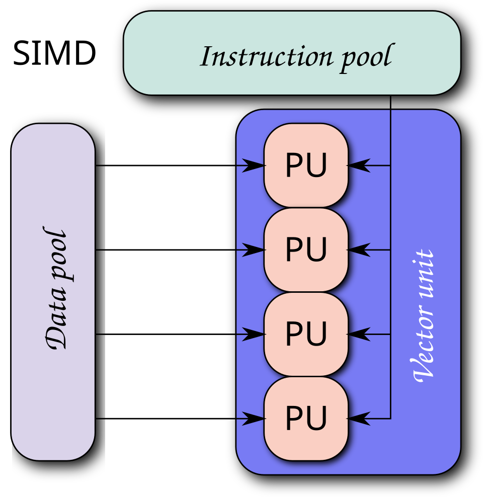
Take a query like the one timed in 6.4, which multiplies two columns and filters on one. For every row, the CPU makes roughly ten virtual calls, each of which first loads a pointer from memory to find out which code to run, and in between it does about one multiply and one add. A modern CPU starts on the next instructions before it knows for certain where the code goes, and the part that guesses is the branch predictor. Every virtual call is one more guess it can get wrong, and a wrong guess throws away the work started on it. The compiler can't help much either. Its usual tricks for fast loops are repeating the loop body to cut loop overhead, and using SIMD instructions, which apply one operation to several values at once. Both need a loop that runs over many values, and here every call handles exactly one row. So the useful arithmetic ends up a small fraction of the instructions the CPU runs.
6.2The interpretation tax, measured in 2005
Peter Boncz, Marcin Zukowski and Niels Nes measured this cost in the MonetDB/X100 paper (CIDR 2005). They profiled MySQL on TPC-H Query 1, a standard benchmark query that scans and aggregates a large table, and found that the five operations doing the query's real work "correspond to only 10% of total execution time". Another 28% went to the aggregation hash table, and the remaining 62% to functions that navigate MySQL's record format.
A CPU's speed at a job is often given as instructions per cycle, abbreviated IPC: how many instructions it finishes, on average, per tick of its clock. In MySQL a single addition took 38 instructions at an IPC of 0.8, fewer than one instruction a tick, so about 49 cycles for one addition. The same CPU could do one multiply every 3 cycles. Their fix kept the Volcano structure but made next() return a vector instead of a row: a small array of values from one column, about a thousand at a time. Every operation then became a tight loop over arrays.
6.3Vectors in DuckDB
DuckDB is built on that idea, and its vector size is a compile-time constant:
namespace duckdb {

//! The default standard vector size
#define DEFAULT_STANDARD_VECTOR_SIZE 2048U

//! The vector size used in the execution engine
#ifndef STANDARD_VECTOR_SIZE
#define STANDARD_VECTOR_SIZE DEFAULT_STANDARD_VECTOR_SIZE
#endif

#if (STANDARD_VECTOR_SIZE & (STANDARD_VECTOR_SIZE - 1) != 0)
#error The vector size must be a power of two
#endif

} // namespace duckdb
One aside on the #if check in that file. In C, != binds tighter than &, so the expression computes N & ((N - 1) != 0), which comes out as N & 1. It catches odd sizes, and a size like 6 would slip through.
Every operator in DuckDB passes a DataChunk of up to 2,048 rows, one vector per column. A filter doesn't copy the rows that pass. It produces a selection vector, a list of the positions that passed, and the next operator reads the values through that list. Our eight amounts fit in a single vector, so we can watch both ways of running the plan side by side. First comes the Volcano way, one value per round trip, and then the vector way, with the whole batch handled by one call per operator:
The vector way did the same work as the Volcano way, but each operator was called once for the batch, and the filter and the sum each became a single loop over an array. A loop like that is exactly what the CPU and the compiler are good at.
6.4Volcano against vectors, side by side
Eight values can't show a speed difference, so here is the same plan over 20 million rows of two in-memory columns, written both ways in C++. The query is SELECT sum(price*qty) WHERE qty < 25, which has the same shape as ours with a multiply added. The Volcano version uses a virtual next() and a virtual expression tree. Its vectorized twin runs two primitives for each batch, a primitive being one tight loop that does one job. The first, sel_lt, is a selection, and the second, sum_mul_sel, multiplies and sums through the selection vector.
Look at sel_lt. It writes position i into sel[j] on every iteration, and advances j only when col[i] < k is true, because a comparison evaluates to 1 or 0. That makes the loop branch-free: there is no if for the CPU to mispredict, and the compiler can pipeline it. The block shows the vectorized half and the loop that feeds it batches of vs values.
// Vectorized primitives: tight loops the compiler can pipeline.
size_t sel_lt(const int32_t* col, int32_t k, size_t n, uint32_t* sel) {
  size_t j = 0;
  for (size_t i = 0; i < n; i++) { sel[j] = i; j += col[i] < k; }   // no branch
  return j;
}
double sum_mul_sel(const double* a, const int32_t* b, const uint32_t* sel, size_t n) {
  double s = 0;
  for (size_t i = 0; i < n; i++) { uint32_t x = sel[i]; s += a[x] * b[x]; }
  return s;
}

for (size_t off = 0; off < N; off += vs) {                 // vs = vector size
  size_t n = std::min(vs, N - off);
  size_t k = sel_lt(&qty[off], 25, n, sel.data());
  total += sum_mul_sel(&price[off], &qty[off], sel.data(), k);
}volcano 233.9 ms 11.69 ns/row sum=6000042453
vector size 1 86.6 ms 4.33 ns/row sum=6000042453
vector size 16 18.9 ms 0.94 ns/row sum=6000042453
vector size 64 16.2 ms 0.81 ns/row sum=6000042453
vector size 2048 18.6 ms 0.93 ns/row sum=6000042453Each line is the median of five runs, and every line prints the same sum, so the versions compute the same thing. The Volcano version spends about 12 ns a row, and batches of 2,048 spend under 1 ns, roughly 12 times less, and repeated runs put the ratio between about 11.7 and 12.6. Even a "vector" of a single row beats Volcano by 2.7 times, because it drops the expression-tree calls.
6.5Why about a thousand and not a million
If batching is good, why not process the whole column in one step? MonetDB, the predecessor of X100, did exactly that, and the X100 paper explains why it wasn't ideal. Every intermediate result becomes a full column in RAM, and the engine ends up running at memory bandwidth instead of cache bandwidth. A cache is a small, fast memory close to the CPU core, and the closest level, L1, holds tens of kilobytes.
A second test makes the intermediates explicit. It runs sum(price * (1 - disc) * (1 + tax)), where each primitive writes its result to a vector, four intermediate vectors of doubles in all. The table shows the median of three runs, with sizes in powers of 1,024:
| Vector size | Intermediates in flight | Time, 20M rows | ns per row |
|---|---|---|---|
| 1 | 32 B | 72.9 ms | 3.6 |
| 128 | 4 KB | 14.8 ms | 0.74 |
| 1,024 | 32 KB | 13.4 ms | 0.67 |
| 2,048 | 64 KB | 13.1 ms | 0.66 |
| 65,536 | 2 MB | 21.2 ms | 1.06 |
| 4,194,304 | 128 MB | 38.3 ms | 1.92 |
| 20,000,000 (whole column) | 610 MB | 36.2 ms | 1.81 |
The fastest sizes were 128 to 2,048 values, where all four intermediates take between 4 KB and 64 KB and stay in the cache levels closest to the core. Past that, each primitive writes its output to a deeper cache level or to DRAM, and the next primitive reads it back. Whole-column processing was 2.8 times slower than the sweet spot. The X100 paper found the same shape on 2005 hardware: vector sizes "between 128 and 8K" worked well, with performance falling once "intermediate results do not fit in the cache anymore".
Where does SIMD come in? Tight loops over arrays are what compilers turn into SIMD instructions automatically. Recompiling the same test with -fno-vectorize -fno-slp-vectorize, which switches that off, took the 2,048 case from 13.1 ms to 35.2 ms, and the binary went from 28 NEON instructions (fmul.2d, fadd.2d, fsub.2d, ARM's SIMD operations) to none. Volcano gets no such help, because no function loops over rows.
6.6The other answer: compile the query
Vectorization isn't the only fix for the per-row overhead. Data-centric code generation, from Thomas Neumann's HyPer, a research database built at TU Munich, compiles the whole pipeline into one tight loop per query, so a row stays in CPU registers from scan to aggregate. Kersten et al. built both approaches inside one engine to compare them (VLDB 2018) and found "both are efficient, but have different strengths": vectorization "is better at hiding cache miss latency", while compilation "requires fewer CPU instructions, which benefits cache-resident workloads".
| Engine | Execution model |
|---|---|
| DuckDB, ClickHouse, Velox, DataFusion, Snowflake | Vectorized |
| HyPer, Umbra, Spark's whole-stage codegen | Compiled |
| Postgres, MySQL, SQLite | Tuple-at-a-time (Postgres adds JIT, compiling code while the query runs, for expressions) |
Whichever model runs the plan, our scene left one question open. The filter produced positions, and the other columns still have to be glued back into rows at some point.
07When to put rows back together
A column store has to hand back rows eventually, because that's what a query returns, so it must decide when to glue the columns back together. Building a row out of its separate columns is called materialization, and the choice is between doing it early and doing it late.
7.1Early and late, step by step
Take SELECT country FROM orders WHERE user_id = 30 on our eight orders. The filter touches only user_id, and the answer needs only country. On the real table, the same shape is SELECT url FROM events WHERE user_id = 12345, where ten rows match out of ten million.
- Early materialization reads the
user_idandcountrycolumns together, builds a (user_id, country) pair for every row, and then filters the pairs. On the real table it decodes ten million URLs to return ten. - Late materialization works on positions for as long as possible:
7.2Timings on the Parquet file
Here is the real table, with the real url column, measured with four threads:
| Query, DuckDB 4 threads | Median |
|---|---|
| SELECT user_id WHERE user_id = 12345 | 6 ms |
| SELECT url WHERE user_id = 12345 | 29–33 ms |
| SELECT sum(length(url)), every url decoded | 115 ms |
Fetching url for ten rows costs far less than decoding the whole column, but it isn't free: about 25 ms over the filter alone. Parquet pages are compressed as a unit, so to reach the one entry you need, the reader still has to decompress the page that holds it.
?So is late materialization always better?
No. Abadi, Myers, DeWitt and Madden studied exactly this in C-Store (ICDE 2007). A predicate is selective when few rows pass it, and their heuristic uses that word: late materialization wins "if output data is aggregated, or if the query has low selectivity (highly selective predicates), or if input data is compressed using a light-weight compression technique". Otherwise, "for high selectivity, non-aggregated, non-compressed data, early materialization should be used", because going back for each column re-reads blocks.
The practical lesson is to put the selective predicate on a small, well-encoded column when you can, so the expensive column is fetched only where rows matched. ClickHouse builds this into its SQL as PREWHERE, a filter stage that reads only the filter's columns first and fetches the other columns only for the granules (blocks of rows, section 8.2) where something matched. You rarely have to write it yourself: by default ClickHouse moves suitable WHERE conditions into PREWHERE on its own.
That finishes the ideas. Everything so far has been about a file. The same ideas run inside real systems, and the first one we'll look at keeps its storage under its own control.
08ClickHouse: MergeTree, parts and granules
Parquet is a file format, and a file can't decide how to batch new data or when to tidy it up. ClickHouse is a server, a program that owns its storage and answers queries over the network, so it can. Its main table engine, MergeTree, borrows an idea from LSM trees (log-structured merge trees), where new data is written as small immutable sorted files that background work merges into bigger ones, and puts a small index on top (8.2). The engine's design is described in the VLDB 2024 paper.
Here are the same 10 million rows, loaded with clickhouse local, the command-line tool that runs the engine without a server. LowCardinality(String) is ClickHouse's wrapper that stores strings through a dictionary, like Parquet's. ORDER BY in a MergeTree table sets the sort order of rows inside every piece of storage, which, as section 4.4 showed, decides what compresses and what can be skipped.
CREATE TABLE events (
  ts DateTime, user_id UInt32,
  country LowCardinality(String), event_type LowCardinality(String),
  amount Float64, url String
) ENGINE = MergeTree ORDER BY (country, event_type, ts);

INSERT INTO events
SELECT ts, user_id, country, event_type, amount, url FROM file('events_snappy.parquet');8.1Every INSERT is a part
A MergeTree table is a set of parts. Each batch of rows that arrives in one INSERT is sorted by the table's ORDER BY and written as a new, immutable part: a directory with one data file and one mark file per column, plus a small primary index file (8.2 explains marks and the index). Background threads merge small parts into bigger ones. A part's name encodes its history, and the steps below show three inserts and the merge that follows:
all_1_1_0: partition all (the table has no partitioning, so everything is in one), blocks 1 to 1, merge level 0.Those are real part names, as listed by system.parts, the built-in table where ClickHouse lists every part, for three small inserts made with merges paused and then resumed. The 10-million-row load arrived as 10 insert blocks, one per Parquet row group, and merged through all_1_6_1 to all_1_10_2.
Why write a new part instead of updating in place? Because every column is sorted and compressed in blocks. Changing one row in place would mean decompressing, editing and recompressing a block in every column file. Writing a new part is a sequential append, and merging later amortises the sort, the same trade an LSM tree makes.
8.2Granules and the sparse primary index
Inside a part, rows are grouped into granules of 8,192 rows. A B-tree index would hold one entry per row, which for ten million rows is ten million entries. ClickHouse's primary index stores the ORDER BY key of the first row of each granule, and nothing else. An index with an entry for only some of the rows is called sparse. The granule size is a setting:
    DECLARE(UInt64, index_granularity, 8192, R"(
    Maximum number of data rows between the marks of an index. I.e how many rows
    correspond to one primary key value.
    )", 0) \
    /* ... */
    DECLARE(UInt64, index_granularity_bytes, 10 * 1024 * 1024, R"(
    Maximum size of data granules in bytes.

    To restrict the granule size only by number of rows, set to `0` (not recommended).
    )", 0) \
For the merged part, system.parts reports:
name        rows      marks  primary_key_bytes_in_memory  compressed  uncompressed
all_1_10_2  10000000  1222   7.32 KiB                     140.70 MiB  532.01 MiB
Ten million rows make 1,221 granules (10,000,000 / 8,192, rounded up) plus a final mark, and the index is only 7.32 KiB, small enough to live in memory permanently.
?How does a sparse index find a row?
It doesn't find rows, it finds granules. A binary search over the 1,221 first keys gives the range of granules that could hold the key, and ClickHouse reads those granules in full. The mark files map each granule number to an offset in each column's compressed data file, so it can seek straight to granule 400 of amount without reading granules 0 to 399.
That design has a price, and it's the same one we met in 2.5. A lookup by a key that isn't the leading ORDER BY column can't be narrowed down by a sparse index, so the query reads every granule. Even a perfect hit reads 8,192 rows to return one. For "fetch order by id", keep a row store.
8.3What ORDER BY buys: counting granules
EXPLAIN indexes = 1 reports how many granules survive the index:
EXPLAIN indexes=1 SELECT sum(amount) FROM events WHERE country='JP' AND event_type='buy';
      PrimaryKey
          Keys: country, event_type
          Granules: 32/1221
          Search Algorithm: binary search

EXPLAIN indexes=1 SELECT sum(amount) FROM events WHERE ts >= '2026-06-01' AND ts < '2026-06-02';
      PrimaryKey
          Keys: ts
          Granules: 81/1221
          Search Algorithm: generic exclusion search
        Ranges: 79
A filter on the first two key columns reads 32 granules, 262,144 rows, to find 249,926 matches. That is 2.6% of the table read. A filter on ts, third in the key, still narrows the read to 81 granules, because within each of the 40 (country, event_type) groups ts is sorted. But it has to test granule ranges instead of running a single binary search, and it reads 79 separate ranges.
| Filter on | Position in ORDER BY | Granules read | Why |
|---|---|---|---|
country, event_type | 1st and 2nd | 32 / 1,221 | One contiguous range, binary search |
ts | 3rd | 81 / 1,221 | Sorted only within each prefix group |
user_id | not in key | 1,221 / 1,221 | No order to exploit |
Sorting by (country, event_type, ts) also compressed the two low-cardinality columns to 11 KiB and 12 KiB for 10 million rows, which is the ClickHouse version of what 4.4 did in Parquet.
8.4Too many parts
Parts are cheap to create and expensive to query in large numbers, because every query must open and merge them all. ClickHouse protects itself with two thresholds per partition, a partition being an independent set of parts, usually split by month or tenant:
    DECLARE(UInt64, parts_to_delay_insert, 1000, R"(
    If the number of active parts in a single partition exceeds the
    `parts_to_delay_insert` value, an `INSERT` is artificially slowed down.
    /* ... */
    DECLARE(UInt64, parts_to_throw_insert, 3000, R"(
    If the number of active parts in a single partition exceeds the
    `parts_to_throw_insert` value, `INSERT` is interrupted with the `Too many
    parts (N). Merges are processing significantly slower than inserts`
    exception.
    /* ... */
    Prior to version 23.6 this setting was set to 300.
Usually the cause is an application inserting one row per request. Each insert is a part, and a thousand requests a second outruns any merge scheduler. The fix is to batch before ClickHouse: buffer in the client and insert every second or every 10,000 rows, put Kafka, a durable log of messages, in front and consume in batches, or turn on async_insert, which makes the server buffer small inserts into one part. The guidance in the MergeTree docs is the same: fewer, larger inserts.
ClickHouse is a server you have to run and operate, and much of this section was about keeping it healthy. That's worth it for many users and many queries, but overkill for one person exploring a Parquet file.
09DuckDB: an analytical engine in your process
DuckDB makes the opposite deployment choice from ClickHouse. It's a library, like SQLite: no server, no network, linked into your Python, R, Node or Java process (SIGMOD 2019 demo).
9.1What's inside
Internally it's the machinery from sections 4 to 7:
| Piece | In DuckDB |
|---|---|
| Storage | Its own single-file format, in row groups of 122,880 rows (DEFAULT_ROW_GROUP_SIZE in storage_info.hpp), which is 60 vectors of 2,048 |
| Skipping | Min/max zonemaps per row group, and the Parquet footer statistics when reading Parquet |
| Execution | Vectorized, 2,048-row DataChunks, selection vectors |
| Parallelism | Morsel-driven (Why DuckDB), after Leis et al. (SIGMOD 2014): threads take the next chunk of rows from a shared scan |
| Files | Queries Parquet, CSV and JSON directly, locally or over HTTP and S3 |
?Why embed an analytical engine instead of running a server?
Because moving data is often the slowest part of analysis. A DataFrame (the in-memory table of pandas or Polars) or a local Parquet file can be scanned in place, with no converting to bytes and sending over a network connection. That's the DuckDB paper's argument for data-science work. You pay what SQLite users pay: one process writes at a time, and it isn't built for many concurrent users.
9.2Choosing an engine
With the pieces in hand, the choice between them follows from the workload:
| Need | Reach for | Why |
|---|---|---|
| Analytics on files on your laptop or in a job | DuckDB | No server, reads Parquet in place |
| Real-time analytics, many concurrent queries, continuous ingest | ClickHouse | A server built for it: MergeTree storage, copies of the data on several machines, and queries spread across them |
| Petabytes on S3 with many engines reading the same data | Parquet (or a table format such as Iceberg, which tracks which files make up a table) plus Trino, Spark or DuckDB | The file format is the shared contract |
| Transactions, point lookups, joins on keys | Postgres | Row store; see chapter 21 |
| Analytics that must be in the same database as the transactions | Postgres replica with a columnar extension, or change data capture (streaming every committed change out of the database) into ClickHouse | Keeps OLTP load off the analytics path |
Once one of these is running, the remaining question is how to tell whether the tricks are working.
10Running analytical engines in production
10.1Where to look
Each question the chapter raised has a command that answers it.
# What did the writer do to each column? (sections 3 and 4)
python3 -c "import pyarrow.parquet as pq; print(pq.ParquetFile('f.parquet').metadata.row_group(0))"
duckdb -c "SELECT path_in_schema, encodings, total_compressed_size, stats_min, stats_max
           FROM parquet_metadata('f.parquet') WHERE row_group_id = 0"

# Where does the time go in a query? (section 6)
duckdb -c "EXPLAIN ANALYZE SELECT ..."          # rows and time per operator

# How many granules did the index leave, and how many parts are there? (section 8)
clickhouse client -q "EXPLAIN indexes = 1 SELECT ..."
clickhouse client -q "SELECT table, count() FROM system.parts WHERE active GROUP BY table"

# What did recent queries read? (sections 5 and 8)
clickhouse client -q "SELECT query_duration_ms, read_rows, read_bytes, query
                      FROM system.query_log ORDER BY event_time DESC LIMIT 10"
read_rows against the rows the query needed is the single best measure of whether your sort key is working.
10.2Rules that hold up
- Name the columns you need. Projection is the biggest skip, and
SELECT *gives it up. - Choose the write order from your filters. Sort files, or the
ORDER BYof a MergeTree table, by the columns your queries filter on, and the same choice also decides what compresses. - Tell the writer about sorted numbers. Timestamps and ids go to delta encoding, and the footer's per-column sizes show whether it worked.
- Write in big batches. Files of hundreds of MB, inserts of thousands of rows, and compact small files after streaming writers.
- Measure the compressor on your read path. Snappy and zstd trade CPU against bytes, and which wins depends on where the bytes come from.
- Compare rows read with rows needed. A large gap says the data isn't clustered the way the queries need.
10.3What you trade for what
| You get | You pay | When the bill arrives |
|---|---|---|
| Queries read only the columns they name | One seek per column to rebuild a row, and slow single-row writes | When someone runs WHERE id = ? or inserts one row per request |
| Columns shrink by large factors | The sort order picks which columns compress; ts grew from 64.6 MB to 69.9 MB when sorted by country | When a column you didn't sort by gets bigger |
| Whole row groups skipped by min and max | Only clustered columns benefit; files are sorted for one set of filters | When a filter on a random column reads every group |
| Vectors cut the per-row cost about 12 times | Each step's output must stay in cache | When batches get so big that whole-column processing is 2.8 times slower |
| zstd makes the file 144 MB instead of 224 MB | More CPU to decompress | When the files sit on a fast local disk |
| One part per insert, merged later | Part count grows with insert rate | As Too many parts |
10.4Symptom, cause, fix
| Symptom | Likely cause | Fix |
|---|---|---|
| Query reads almost every row group or granule despite a narrow filter | Filter column isn't clustered; min/max ranges overlap | Sort files or ORDER BY on the filter columns; add a page index or Bloom filter for equality |
| Many small files, slow listing and scans | Streaming writer flushing every few seconds | Compact into files of hundreds of MB |
Too many parts on insert | Row-at-a-time inserts | Batch client-side, async_insert, or a queue in front |
| A column is far bigger than expected | Dictionary fell back to plain; wrong encoding for sorted data | Check per-chunk sizes; delta-encode sorted ints; zstd |
| Queries fast on one thread, not faster on more | Too few row groups after skipping, or one giant row group | Smaller row groups, more files, balanced partitions |
SELECT * dashboards slow and expensive | Every column read and decoded | Name the columns |
| Point lookups slow on ClickHouse | Key isn't the leading ORDER BY column; granule reads 8,192 rows | Keep lookups in a row store, or add a projection (a hidden copy of the table sorted in a different order) |
11Summary
- Columns win when queries touch few columns of many rows. Our eight orders needed 16 of 32 values, and on the real table
sum(amount)read 26 MB of Parquet instead of an 804 MB SQLite file. - Parquet is file, row group, column chunk, page, with metadata last. The footer holds positions and min and max for every chunk, 7,940 bytes for 10M rows.
- Encoding comes before compression. Ten countries packed to 4 bits a value, and a sorted timestamp delta-encoded from 64.55 MB to 0.07 MB.
- Dictionaries fail on high-cardinality columns. Past pyarrow's 1 MB cap the writer falls back to plain, and the dictionary page is wasted.
- Sort order decides compression and skipping. Sorting by country took that column from 5.05 MB to 0.02 MB, and a day filter read one row group of ten.
- Min and max statistics only skip clustered columns. A random
user_idrange read every row group. - Many small files cost more than one big one. The same rows in 1,000 files ran roughly six times slower.
- Volcano spends most of its time interpreting. Vectors of about a thousand values cut the per-row cost roughly 12 times in the C++ test.
- Vectors should fit in cache. 128 to 2,048 values was fastest, and processing whole columns was 2.8 times slower.
- Late materialization fetches wide columns only where rows matched. Ten URLs cost about 30 ms against 115 ms to decode all of them.
- ClickHouse indexes granules, not rows. 8,192 rows per index entry, 7.32 KiB of index for 10 million rows, and one immutable part per insert.
12Build this
A tiny columnar scanner. One table, three columns, about 400 lines of C++ or Rust.
- Write a file format: a header, then for each block of 65,536 rows one contiguous array per column, and a footer with each block's offset and the min and max of each column. Dictionary-encode one string column to
uint8. - Write a scanner that reads the footer, skips blocks whose min and max can't match a filter, and processes the surviving blocks in vectors with a selection vector.
- Measure three things: bytes read with and without the skip, time per row at vector sizes 1, 256, 2,048 and 65,536, and the size of the string column with and without the dictionary. Then sort the data by the filter column and run it again.
If your numbers have the shape of sections 4 to 6, you've built the core of every engine in this chapter.
13Interview questions
beginnerWhy are column stores faster for analytics?›
Analytical queries read a few columns of many rows. A column store reads only those columns, so it moves far fewer bytes. Each column holds one type, so it compresses well, and the engine can process a column as an array in tight loops. On a 10-million-row table, sum(amount) read 26 MB of Parquet where a row store had to read an 804 MB file, and a column engine ran it 36 times faster on one thread.
beginnerWhat's in a Parquet footer, and why is it at the end?›
The schema, and for every row group and column chunk: byte offsets, compressed and uncompressed sizes, encodings, value counts and min, max and null statistics. It's at the end because the writer only knows those values after writing the data, so it can stream row groups and write the index once. Readers fetch the last 8 bytes for the footer length, then the footer, then only the chunks they need.
intermediateA Parquet column is much bigger than you expected. What do you check?›
The per-chunk total_compressed_size and encodings in the footer. Common causes are a high-cardinality string column whose dictionary hit the size cap and fell back to plain, a sorted integer or timestamp stored plain instead of delta-encoded, snappy where zstd would do much better, and rows written in an order that breaks up runs. Rewriting sorted by low-cardinality columns can shrink them by orders of magnitude.
intermediateWhy doesn't a filter on user_id skip any row groups when a filter on ts skips nine of ten?›
Skipping uses per-row-group min and max. ts was written in order, so each group covers a narrow, non-overlapping time range, and a one-day filter matches one group. The user_id values are scattered, so every group's range spans nearly the whole domain and nothing can be ruled out. Fix it by sorting on the filter column when writing, or add a page index or Bloom filter for equality lookups.
intermediateWhat causes ClickHouse's 'Too many parts' error?›
Each INSERT creates an immutable part, and background merges combine them. If inserts arrive faster than merges can keep up, usually from one-row inserts per request, the active part count in a partition passes parts_to_delay_insert (1,000), where inserts get slowed, and then parts_to_throw_insert (3,000), where they're rejected. Batch inserts client-side, use async_insert, or put a queue in front.
deepExplain vectorized execution. Why around a thousand values per vector and not the whole column?›
Volcano returns one row per virtual next() call and interprets expressions per row, so most instructions are overhead: the X100 paper found MySQL spending about 10% of TPC-H Q1 on real work. Vectorized engines return batches and run each operation as a loop over arrays, which spreads the call overhead over the batch and lets the compiler pipeline and SIMD-vectorize. But each primitive materializes its output, so vectors must be small enough that all intermediates stay in cache. Too large and each step round-trips through memory, which is the column-at-a-time problem MonetDB had. In a test over 20 million rows, 128 to 2,048 values was fastest, and whole-column processing was 2.8 times slower.
deepWhen is late materialization worse than early?›
When many rows pass the filter and the output isn't aggregated. Late materialization keeps positions and goes back to fetch other columns, which means re-reading and re-decompressing blocks. Abadi et al.'s heuristic from C-Store: use late materialization when output is aggregated, predicates are highly selective, or data uses lightweight compression. Otherwise early materialization can win.
deepHow does ClickHouse's sparse primary index differ from a B-tree, and what does it cost?›
A B-tree has one entry per row and finds a row exactly. ClickHouse stores the key of the first row of each 8,192-row granule: 1,221 entries for 10 million rows, 7.32 KiB, always in memory. It binary-searches to a range of granules and reads them whole, with mark files mapping granule numbers to offsets in each column file. The costs are that point lookups read at least 8,192 rows, and filters on columns that aren't a prefix of ORDER BY skip poorly or not at all.
14Go deeper
SELECT count(*) on a 10-million-row Parquet file took 0.3 ms. Why?›
The row count of every row group is in the footer, so the engine answers from metadata and never reads a data page.
A column with 10 distinct values in a 1,048,576-row group took 529,155 bytes. Where does that come from?›
Dictionary encoding with RLE/bit-packed indexes: 10 values need 4 bits, and 1,048,576 × 4 bits is 524,288 bytes. The rest is the dictionary and page headers.
Why did a one-day filter get slower going from 1 thread to 4?›
Skipping left one row group, and a row group is the unit of parallel work. The extra threads had nothing to do but still cost setup.
Your ClickHouse table is ORDER BY (tenant, ts). A query filters only on ts. Does the index help?›
Somewhat. ts is sorted inside each tenant's range, so generic exclusion
search can skip granules, but it reads many separate ranges instead of one.
On the 10-million-row table, a third-position ts filter read 81 of 1,221
granules.
The paper behind vectorized execution. The MySQL profile in section 6.2 and the vector-size experiment in section 6.5 repay a full read.
Early versus late materialization, with an analytical model and the heuristic quoted in section 7.
The column-store design that Vertica came from: sorted projections, compression-aware operators, a write store in front of a read store.
The spec itself. Read ColumnMetaData, Statistics and PageHeader, then
the encodings document for the RLE/bit-packing hybrid.
MergeTree, parts, granules, the vectorized engine and the integration layer, from the people who built them.
A long, concrete walk through granules, marks and index selection with
EXPLAIN output, including why the order of key columns matters.
Both execution models inside one engine, compared fairly, with SIMD and multi-core results.
Where Parquet's nested encoding with repetition and definition levels comes from.
15Related chapters
Cache lines and cache sizes, the reason vectors of about a thousand values beat whole columns. Chapter 02.
Pipelines, branch prediction and SIMD, the machinery vectorized primitives are written for. Chapter 01.
The row store on the other side of the comparison: the heap, tuples and pages. Chapter 21.
How events usually reach an analytical store in batches big enough to avoid small files and too many parts. Chapter 23.